Hole Filling

"Make it Real"

A Lithograph of a Waterfall

A Lithograph of a Skull

An Oil Painting of an Old Man

An Oil Painting of People Around a Fire

HW5 Part A: The Power of Diffusion Models!

COMS4732: Computer Vision 2

Part B

Due: Friday, April 17 11:59pm PT

We recommend using GPUs from Colab to finish this project!
(students get Colab Pro for free)!

Starter code can be found here.

Collapse all

Overview

In part A you will play around with diffusion models, implement diffusion sampling loops, and use them for other tasks such as inpainting and creating optical illusions. Instructions can be found below and in the starter code above.

Because part A is simply to get your feet wet with pre-trained diffusion models, all deliverables should be completed in the notebook. You will still submit a webpage with your results.

Note: Implementations are provided for parts 1.1, 1.2, 1.3, and 1.4. You can find versions of the starter code with and without these parts implemented at the link above. You are still expected to submit images for those sections but are just not required to implement them yourselves.

Part 0: Setup

Gaining Access to DeepFloyd

We are going to use the DeepFloyd IF diffusion model. DeepFloyd is a two stage model trained by Stability AI. The first stage produces images of size $64 \times 64$ and the second stage takes the outputs of the first stage and generates images of size $256 \times 256$. We provide upsampling code at the very end of the notebook, though this is not required in your submission. Before using DeepFloyd, you must accept its usage conditions. To do so:

1. Make a Hugging Face account and log in.
2. Accept the license on the model card of DeepFloyd/IF-I-XL-v1.0. For affiliation, you can fill in "Columbia University" Accepting the license on the stage I model card will auto accept for the other IF models.
3. Log in locally by entering your Hugging Face Hub access token below. You should be able to find and create tokens here. A read token is enough for this project.

Play with the Model using Your Own Text Prompts!

DeepFloyd was trained as a text-to-image model, which takes text prompts as input and outputs images that are aligned with the text. However, a raw text string cannot be directly used as the model's input — we first need to convert it into a high-dimensional vector (of 4096 dimensions in our case) that the model can understand, a.k.a. prompt embeddings.

Since prompt encoders are always very big and hard to run in your notebook, we provide two Huggingface clusters A and B for generating your own prompt embeddings! Both are the same and feel free to use either of them. Please follow their instructions to create a dictionary of embeddings for your prompts, download the resulting .pth file, and load it in Google Colab.

Please note that both clusters have daily usage limits, so if you're unable to use one, please try another or try again tomorrow. Alternatively, START EARLY and download the .pth file in advance — you only need to generate it once, and you can reuse the downloaded file afterward. If the official site experiences issues or runs out of computation, you can download one of our precomputed embeddings, but this is a predefined set of prompts and lacks flexibility. We want to see your creativity!

Deliverables

• Come up with some interesting text prompts and generate their embeddings.
• Choose 3 of your prompts to generate images and display the caption and the output of the model. Reflect on the quality of the outputs and their relationships to the text prompts. Make sure to try at least 2 different num_inference_steps values.
• Report the random seed that you're using here. You should use the same seed all subsequent parts.

Hint

• Since we ask you to generate visual anagrams and hybrid images, you may want to include several text pairs that you plan to use for those tasks later.

Part 1: Sampling Loops

In this part of the problem set, you will write your own “sampling loops” that use the pretrained DeepFloyd denoisers. These should produce high quality images such as the ones generated above.

You will then modify these sampling loops to solve different tasks such as inpainting or producing optical illusions.

Diffusion Models Primer

Starting with a clean image, $x_0$, we can iteratively add noise to an image, obtaining progressively more and more noisy versions of the image, $x_t$, until we're left with basically pure noise at timestep $t=T$. When $t=0$, we have a clean image, and for larger $t$ more noise is in the image.

A diffusion model tries to reverse this process by denoising the image. By giving a diffusion model a noisy $x_t$ and the timestep $t$, the model predicts the noise in the image. With the predicted noise, we can either completely remove the noise from the image, to obtain an estimate of $x_0$, or we can remove just a portion of the noise, obtaining an estimate of $x_{t-1}$, with slightly less noise.

To generate images from the diffusion model (sampling), we start with pure noise at timestep $T$ sampled from a gaussian distribution, which we denote $x_T$. We can then predict and remove part of the noise, giving us $x_{T-1}$. Repeating this process until we arrive at $x_0$ gives us a clean image.

For the DeepFloyd models, $T = 1000$.

The exact amount of noise added at each step is dictated by noise coefficients, $\bar\alpha_t$, which were chosen by the people who trained DeepFloyd.

1.1 Implementing the Forward Process (Implementation Provided)

A key part of diffusion is the forward process, which takes a clean image and adds noise to it. In this part, we will write a function to implement this. The forward process is defined by:

$$q(x_t | x_0) = N(x_t ; \sqrt{\bar\alpha} x_0, (1 - \bar\alpha_t)\mathbf{I})\tag{A.1}$$

which is equivalent to computing $$ x_t = \sqrt{\bar\alpha_t} x_0 + \sqrt{1 - \bar\alpha_t} \epsilon \quad \text{where}~ \epsilon \sim N(0, 1) \tag{A.2}$$ That is, given a clean image $x_0$, we get a noisy image $ x_t $ at timestep $t$ by sampling from a Gaussian with mean $ \sqrt{\bar\alpha_t} x_0 $ and variance $ (1 - \bar\alpha_t) $. Note that the forward process is not just adding noise -- we also scale the image.

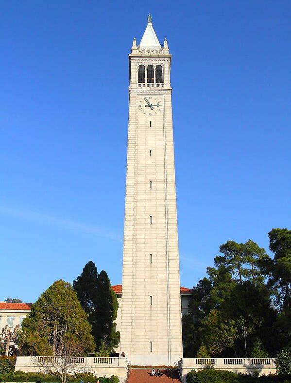
You will need to use the alphas_cumprod variable, which contains the $\bar\alpha_t$ for all $t \in [0, 999]$. Remember that $t=0$ corresponds to a clean image, and larger $t$ corresponds to more noise. Thus, $\bar\alpha_t$ is close to 1 for small $t$, and close to 0 for large $t$. The test image of the Campanile can be downloaded at here, which you should then resize to 64x64. Run the forward process on the test image with $t \in [250, 500, 750]$ and display the results. You should get progressively more noisy images.

Deliverables

• Implement the noisy_im = forward(im, t) function
• Show the Campanile at noise level [250, 500, 750].

Hints

• The torch.randn_like function is helpful for computing $\epsilon$.
• Use the alphas_cumprod variable, which contains an array of the hyperparameters, with alphas_cumprod[t] corresponding to $\bar\alpha_t$.

Berkeley Campanile

Noisy Campanile at t=250

Noisy Campanile at t=500

Noisy Campanile at t=750

1.2 Classical Denoising (Implementation Provided)

Let's try to denoise these images using classical methods. Again, take noisy images for timesteps [250, 500, 750], but use Gaussian blur filtering to try to remove the noise. Getting good results should be quite difficult, if not impossible.

Deliverables

• For each of the 3 noisy Campanile images from the previous part, show your best Gaussian-denoised version side by side.

Hint:

• torchvision.transforms.functional.gaussian_blur is useful. Here is the documentation.

Noisy Campanile at t=250

Noisy Campanile at t=500

Noisy Campanile at t=750

Gaussian Blur Denoising at t=250

Gaussian Blur Denoising at t=500

Gaussian Blur Denoising at t=750

1.3 One-Step Denoising (Implementation Provided)

Now, we'll use a pretrained diffusion model to denoise. The actual denoiser can be found at stage_1.unet. This is a UNet that has already been trained on a very, very large dataset of $(x_0, x_t)$ pairs of images. We can use it to recover Gaussian noise from the image. Then, we can remove this noise to recover (something close to) the original image. Note: this UNet is conditioned on the amount of Gaussian noise by taking timestep $t$ as additional input.

Because this diffusion model was trained with text conditioning, we also need a text prompt embedding. We provide the embedding for the prompt "a high quality photo" for you to use. Later on, you can use your own text prompts.

Deliverables

• For the 3 noisy images from 1.2 (t = [250, 500, 750]):
  • Use your forward function to add noise to your Campanile.
  • Estimate the noise in the new noisy image, by passing it through stage_1.unet
  • Remove the noise from the noisy image to obtain an estimate of the original image.
  • Visualize the original image, the noisy image, and the estimate of the original image

Hints

• When removing the noise, you can't simply subtract the noise estimate. Recall that in equation A.2 we need to scale the noise. Look at equation A.2 to figure out how we predict $x_0$ from $x_t$ and $t$.
• You will probably have to wrangle tensors to the correct device and into the correct data types. The functions .to(device) and .half() will be useful. The denoiser is loaded on the device cuda as half precision (to save memory), so inputs to the denoiser need to match them.
• The signature for the unet is stage_1.unet(im_noisy, t, encoder_hidden_states=prompt_embeds, return_dict=False). You need to pass in the noisy image, the timestep, and the prompt embeddings. The return_dict argument just makes the output nicer.
• The unet will output a tensor of shape (1, 6, 64, 64). This is because DeepFloyd was trained to predict the noise as well as variance of the noise. The first 3 channels is the noise estimate, which you will use. The second 3 channels is the variance estimate which you may ignore.
• To save GPU memory, you should wrap all of your code in a with torch.no_grad(): context. This tells torch not to do automatic differentiation, and saves a considerable amount of memory.

Noisy Campanile at t=250

Noisy Campanile at t=500

Noisy Campanile at t=750

One-Step Denoised Campanile at t=250

One-Step Denoised Campanile at t=500

One-Step Denoised Campanile at t=750

1.4 Iterative Denoising (Implementation Provided)

In part 1.3, you should see that the denoising UNet does a much better job of projecting the image onto the natural image manifold, but it does get worse as you add more noise. This makes sense, as the problem is much harder with more noise!

But diffusion models are designed to denoise iteratively. In this part we will implement this.

In theory, we could start with noise $x_{1000}$ at timestep $T=1000$, denoise for one step to get an estimate of $x_{999}$, and carry on until we get $x_0$. But this would require running the diffusion model 1000 times, which is quite slow (and costs $$$).

It turns out, we can actually speed things up by skipping steps. The rationale for why this is possible is due to a connection with differential equations. It's a tad complicated, and not within scope for this course, but if you're interested you can check out this excellent article.

To skip steps we can create a new list of timesteps that we'll call strided_timesteps, which does just this. strided_timesteps[0] will correspond to the the largest $t$ (and thus the noisiest image) and strided_timesteps[-1] will correspond to $t = 0$ (and thus a clean image). One simple way of constructing this list is by introducing a regular stride step (e.g. stride of 30 works well).

On the ith denoising step we are at $ t = $ strided_timesteps[i], and want to get to $ t' =$ strided_timesteps[i+1] (from more noisy to less noisy). To actually do this, we have the following formula:

\[x_{t'} = \frac{\sqrt{\bar\alpha_{t'}}\beta_t}{1 - \bar\alpha_t} x_0 + \frac{\sqrt{\alpha_t}(1 - \bar\alpha_{t'})}{1 - \bar\alpha_t} x_t + v_\sigma\tag{A.3}\]

where:

• $x_t$ is your image at timestep $t$
• $x_{t'}$ is your noisy image at timestep $t'$ where $t' < t$ (less noisy)
• $\bar\alpha_t$ is defined by alphas_cumprod, as explained above.
• $\alpha_t = \frac{\bar\alpha_t}{\bar\alpha_{t'}}$
• $\beta_t = 1 - \alpha_t$
• $x_0$ is our current estimate of the clean image using one-step denoising

The $v_\sigma$ is random noise, which in the case of DeepFloyd is also predicted. The process to compute this is not very important, so we supply a function, add_variance, to do this for you. </p>

You can think of this as a linear interpolation between the signal and noise:

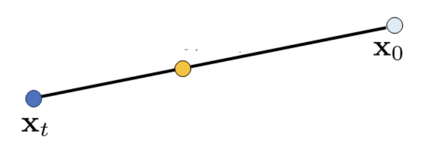
Interpolation

See equations 6 and 7 of the DDPM paper for more information (Denoising Diffusion Probabilistic Models, the paper that introduces the diffusion model, which comes from Cal!). Be careful about bars above the alpha! Some have them and some do not.

First, create the list strided_timesteps. You should start at timestep 990, and take step sizes of size 30 until you arrive at 0. After completing the problem set, feel free to try different "schedules" of timesteps.

Also implement the function iterative_denoise(im_noisy, i_start), which takes a noisy image image, as well as a starting index i_start. The function should denoise an image starting at timestep timestep[i_start], applying the above formula to obtain an image at timestep t' = timestep[i_start + 1], and repeat iteratively until we arrive at a clean image.

Add noise to the test image im to timestep timestep[10] and display this image. Then run the iterative_denoise function on the noisy image, with i_start = 10, to obtain a clean image and display it. Please display every 5th image of the denoising loop. Compare this to the "one-step" denoising method from the previous section, and to gaussian blurring.

Deliverables

Using i_start = 10:

• Create strided_timesteps: a list of monotonically decreasing timesteps, starting at 990, with a stride of 30, eventually reaching 0. Also initialize the timesteps using the function stage_1.scheduler.set_timesteps(timesteps=strided_timesteps)
• Complete the iterative_denoise function
• Show the noisy Campanile every 5th loop of denoising (it should gradually become less noisy)
• Show the final predicted clean image, using iterative denoising
• Show the predicted clean image using only a single denoising step, as was done in the previous part. This should look much worse.
• Show the predicted clean image using gaussian blurring, as was done in part 1.2.

Hints

• Remember, the unet will output a tensor of shape (1, 6, 64, 64). This is because DeepFloyd was trained to predict the noise as well as variance of the noise. The first 3 channels is the noise estimate, which you will use here. The second 3 channels is the variance estimate which you will pass to the add_variance function
• Read the documentation for the add_variance function to figure out how to use it to add the $v_\sigma$ to the image.
• Depending on if your final images are torch tensors or numpy arrays, you may need to modify the `show_images` call a bit.

Noisy Campanile at t=90

Noisy Campanile at t=240

Noisy Campanile at t=390

Noisy Campanile at t=540

Noisy Campanile at t=690

Original

Iteratively Denoised Campanile

One-Step Denoised Campanile

Gaussian Blurred Campanile

1.5 Diffusion Model Sampling

In part 1.4, we use the diffusion model to denoise an image. Another thing we can do with the iterative_denoise function is to generate images from scratch. We can do this by setting i_start = 0 and passing im_noisy as random noise. This effectively denoises pure noise. Please do this, and show 5 results of the prompt"a high quality photo".

Deliverables

• Show 5 sampled images.

Hints

• Use torch.randn to make the noise.
• Make sure you move the tensor to the correct device and correct data type by calling .half() and .to(device).
• The quality of the images will not be spectacular, but should be reasonable images. We will fix this in the next section with CFG.

Sample 1

Sample 2

Sample 3

Sample 4

Sample 5

1.6 Classifier-Free Guidance (CFG)

You may have noticed that the generated images in the prior section are not very good, and some are completely non-sensical. In order to greatly improve image quality (at the expense of image diversity), we can use a technicque called Classifier-Free Guidance.

In CFG, we compute both a conditional and an unconditional noise estimate. We denote these $\epsilon_c$ and $\epsilon_u$. Then, we let our new noise estimate be: $$\epsilon = \epsilon_u + \gamma (\epsilon_c - \epsilon_u) \tag{A.4}$$ where $\gamma$ controls the strength of CFG. Notice that for $\gamma=0$, we get an unconditional noise estimate, and for $\gamma=1$ we get the conditional noise estimate. The magic happens when $\gamma > 1$. In this case, we get much higher quality images. Why this happens is still up to vigorous debate. For more information on CFG, you can check out this blog post.

Please implement the iterative_denoise_cfg function, identical to the iterative_denoise function but using classifier-free guidance. To get an unconditional noise estimate, we can just pass an empty prompt embedding to the diffusion model (the model was trained to predict an unconditional noise estimate when given an empty text prompt).

Disclaimer Disclaimer Before, we used "a high quality photo" as a "null" condition. Now, we will use the actual "" null prompt for unconditional guidance for CFG. In the later part, you should always use "" null prompt for unconditional guidance.

Deliverables

• Implement the iterative_denoise_cfg function
• Show 5 images of "a high quality photo" with a CFG scale of $\gamma=7$. Now this prompt becomes a condition (but fairly weak) to generate conditional noise! You will use your customized prompts as stronger conditions in part 1.7 - part 1.9.

Hints

• You will need to run the UNet twice, once for the conditional prompt embedding, and once for the unconditional
• The UNet will predict both a conditional and an unconditional variance. Just use the conditional variance with the add_variance function.
• The resulting images should be much better than those in the prior section.

Sample 1 with CFG

Sample 2 with CFG

Sample 3 with CFG

Sample 4 with CFG

Sample 5 with CFG

1.7 Image-to-image Translation

Note: You should use CFG from this point forward.

In part 1.4, we take a real image, add noise to it, and then denoise. This effectively allows us to make edits to existing images. The more noise we add, the larger the edit will be. This works because in order to denoise an image, the diffusion model must to some extent "hallucinate" new things -- the model has to be "creative." Another way to think about it is that the denoising process "forces" a noisy image back onto the manifold of natural images.

Here, we're going to take the original Campanile image, noise it a little, and force it back onto the image manifold without any conditioning. Effectively, we're going to get an image that is similar to the Campanile (with a low-enough noise level). This follows the SDEdit algorithm.

To start, please run the forward process to get a noisy Campanile, and then run the iterative_denoise_cfg function using a starting index of [1, 3, 5, 7, 10, 20] steps and show the results, labeled with the starting index. You should see a series of "edits" to the original image, gradually matching the original image closer and closer.

Deliverables

• Edits of the Campanile image, using the given prompt at noise levels [1, 3, 5, 7, 10, 20] with the conditional text prompt "a high quality photo"
• Edits of 2 of your own test images, using the same procedure.

Hints

• You should have a range of images, gradually looking more like the original image

SDEdit with i_start=1

SDEdit with i_start=3

SDEdit with i_start=5

SDEdit with i_start=7

SDEdit with i_start=10

SDEdit with i_start=20

Campanile

1.7.1 Editing Hand-Drawn and Web Images

This procedure works particularly well if we start with a nonrealistic image (e.g. painting, a sketch, some scribbles) and project it onto the natural image manifold.

Please experiment by starting with hand-drawn or other non-realistic images and see how you can get them onto the natural image manifold in fun ways.

We provide you with 2 ways to provide inputs to the model:

1. Download images from the web
2. Draw your own images

Please find an image from the internet and apply edits exactly as above. And also draw your own images, and apply edits exactly as above. Feel free to copy the prior cell here. For drawing inspiration, you can check out the examples on this project page.

Deliverables

• 1 image from the web of your choice, edited using the above method for noise levels [1, 3, 5, 7, 10, 20] (and whatever additional noise levels you want)
• 2 hand drawn images, edited using the above method for noise levels [1, 3, 5, 7, 10, 20] (and whatever additional noise levels you want)

Hints

• We provide you with preprocessing code to convert web images to the format expected by DeepFloyd
• Unfortunately, the drawing interface is hardcoded to be 300x600 pixels, but we need a square image. The code will center crop, so just draw in the middle of the canvas.

Avocado at i_start=1

Avocado at i_start=3

Avocado at i_start=5

Avocado at i_start=7

Avocado at i_start=10

Avocado at i_start=20

Avocado

House at i_start=1

House at i_start=3

House at i_start=5

House at i_start=7

House at i_start=10

House at i_start=20

Original House Sketch

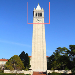
1.7.2 Inpainting

We can use the same procedure to implement inpainting (following the RePaint paper). That is, given an image $x_{orig}$, and a binary mask $\bf m$, we can create a new image that has the same content where $\bf m$ is 0, but new content wherever $\bf m$ is 1.

To do this, we can run the diffusion denoising loop. But at every step, after obtaining $x_t$, we "force" $x_t$ to have the same pixels as $x_{orig}$ where $\bf m$ is 0, i.e.:

$$ x_t \leftarrow \textbf{m} x_t + (1 - \textbf{m}) \text{forward}(x_{orig}, t) \tag{A.5}$$

Essentially, we leave everything inside the edit mask alone, but we replace everything outside the edit mask with our original image -- with the correct amount of noise added for timestep $t$.

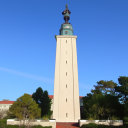
Please implement this below, and edit the picture to inpaint the top of the Campanile.

Deliverables

• A properly implemented inpaint function
• The Campanile inpainted (feel free to use your own mask)
• 2 of your own images edited (come up with your own mask)
  • look at the results from this paper for inspiration

Hints

• Reuse the forward function you implemented earlier to implement inpainting
• Because we are using the diffusion model for tasks it was not trained for, you may have to run the sampling process a few times before you get a nice result.
• You can copy and paste your iterative_denoise_cfg function. To get inpainting to work should only require (roughly) 1-2 additional lines and a few small changes.

Campanile

Mask

Hole to Fill

Campanile Inpainted

1.7.3 Text-Conditional Image-to-image Translation

Now, we will do the same thing as SDEdit, but guide the projection with a text prompt. This is no longer pure "projection to the natural image manifold" but also adds control using language. This is simply a matter of changing the prompt from "a high quality photo" to any of your prompt!

Deliverables

• Edits of the Campanile, using the given prompt at noise levels [1, 3, 5, 7, 10, 20]
• Edits of 2 of your own test images, using the same procedure

Hints

• The images should gradually look more like original image, but also look like the text prompt.

Rocket Ship at noise level 1

Rocket Ship at noise level 3

Rocket Ship at noise level 5

Rocket Ship at noise level 7

Rocket Ship at noise level 10

Rocket Ship at noise level 20

Campanile

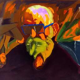
1.8 Visual Anagrams

In this part, we are finally ready to implement Visual Anagrams and create optical illusions with diffusion models. In this part, we will create an image that looks like "an oil painting of people around a campfire", but when flipped upside down will reveal "an oil painting of an old man".

To do this, we will denoise an image $x_t$ at step $t$ normally with the prompt $p_1$, to obtain noise estimate $\epsilon_1$. But at the same time, we will flip $x_t$ upside down, and denoise with the prompt $p_2$, to get noise estimate $\epsilon_2$. We can flip $\epsilon_2$ back, and average the two noise estimates. We can then perform a reverse/denoising diffusion step with the averaged noise estimate.

The full algorithm will be:

$$ \epsilon_1 = \text{CFG of UNet}(x_t, t, p_1) $$

$$ \epsilon_2 = \text{flip}(\text{CFG of UNet}(\text{flip}(x_t), t, p_2)) $$

$$ \epsilon = (\epsilon_1 + \epsilon_2) / 2 $$

where UNet is the diffusion model UNet from before, $\text{flip}(\cdot)$ is a function that flips the image, and $p_1$ and $p_2$ are two different text prompt embeddings. And our final noise estimate is $\epsilon$. Please implement the above algorithm and show example of an illusion.

Deliverables

• Correctly implemented visual_anagrams function
• 2 illusions of your choice that change appearance when you flip it upside down (feel free to take inspirations from this page).

Hints

• You may have to run multiple times to get a really good result for the same reasons as above.

An Oil Painting of an Old Man

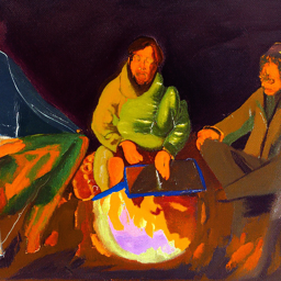
An Oil Painting of People around a Campfire

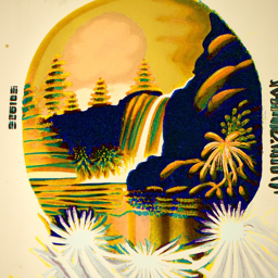
1.9 Hybrid Images

In this part we'll implement Factorized Diffusion and create hybrid images just like in project 2.

In order to create hybrid images with a diffusion model we can use a similar technique as above. We will create a composite noise estimate $\epsilon$, by estimating the noise with two different text prompts, and then combining low frequencies from one noise estimate with high frequencies of the other. The algorithm is:

$ \epsilon_1 = \text{CFG of UNet}(x_t, t, p_1) $

$ \epsilon_2 = \text{CFG of UNet}(x_t, t, p_2) $

$ \epsilon = f_\text{lowpass}(\epsilon_1) + f_\text{highpass}(\epsilon_2)$

where UNet is the diffusion model UNet, $f_\text{lowpass}$ is a low pass function, $f_\text{highpass}$ is a high pass function, and $p_1$ and $p_2$ are two different text prompt embeddings. Our final noise estimate is $\epsilon$. Please show an example of a hybrid image using this technique (you may have to run multiple times to get a really good result for the same reasons as above). We recommend that you use a gaussian blur of kernel size 33 and sigma 2.

Deliverables

• Correctly implemented make_hybrids function
• 2 hybrid images of your choosing (feel free to take inspirations from this page).

Hints

• use torchvision.transforms.functional.gaussian_blur
• You may have to run multiple times to get a really good result for the same reasons as above

Hybrid image of a skull and a waterfall

Bells & Whistles (Optional)

• More visual anagrams! Visual anagrams in part 1.8 are created by flipping images upside down. However, there are much more transformations that also create visual anagrams! Refer to this paper and select two more transformations to create visual anagrams.
• Design a course logo! Doing text-conditioned image-to-image translation on UCB's logo or your drawing may be a good idea.
• Your own ideas: Be creative!

Deliverable Checklist

• Make sure that your website and submission include all the deliverables in each section above.
• Submit your PDF and code to corresponding assignments on Gradescope.

Acknowledgements

This project was a joint effort by Daniel Geng, Ryan Tabrizi, Hang Gao, Jingfeng Yang, and Jameson Crate, advised by Liyue Shen, Andrew Owens, and Alexei Efros.

---

</details>