Homework 4

COMS4732: Computer Vision 2

Neural Radiance Fields!

Due Date: Friday March 27, 11:59pm ET (3 weeks)

Starter code can be found here.

START EARLY! This HW, along with HW5, are by far the most difficult and time-consuming assignments this semester.

Collapse all

Overview

In HW2, we used a simple feature matching procedure to find correspondences between two images. In HW3, we did simple structure from motion (SfM) to estimate the 3D camera poses for 2 images. In this homework, you will use the outputs of an off-the-shelf SfM pipeline (COLMAP) to build a NeRF of your own object.

Note on compute requirements: We’re using PyTorch to implement neural networks with GPU acceleration. If you have an M-series Mac (M1/M2/M3), you should be able to run everything locally using the MPS backend. For older or less powerful hardware, we recommend using GPUs from Colab. Colab Pro is now free for students.

---

Part 1: Fit a Neural Field to a 2D Image

From lecture we know that we can use a Neural Radiance Field (NeRF) (\(F: \{x, y, z, \theta, \phi\} \rightarrow \{r, g, b, \sigma\}\)) to represent a 3D space. But before jumping into 3D, let’s first get familar with NeRF (and PyTorch) using a 2D example. In fact, since there is no concept of radiance in 2D, the Neural Radiance Field falls back to just a Neural Field (\(F: \{u, v\} \rightarrow \{r, g, b\}\)) in 2D, in which \(\{u, v\}\) is the pixel coordinate. In this section, we will create a neural field that can represent a 2D image and optimize that neural field to fit this image. You can start from this image, but feel free to try out any other images.

[Impl: Network] You would need to create an Multilayer Perceptron (MLP) network with Sinusoidal Positional Encoding (PE) that takes in the 2-dim pixel coordinates, and output the 3-dim pixel colors.

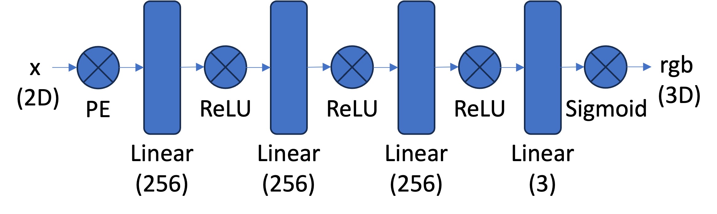
• Multilayer Perceptron (MLP): An MLP is simply a stack of non linear activations (e.g., torch.nn.ReLU() or torch.nn.Sigmoid()) and fully connected layers (torch.nn.Linear()). For this part, you can start from building an MLP with the structure shown in the image below. Note that you would need to have a Sigmoid layer at the end of the MLP to constrain the network output be in the range of (0, 1), as a valid pixel color (don’t forget to also normalize your image from [0, 255] to [0, 1] when you use it for supervision!). You can take a reference from this tutorial on how to create an MLP in PyTorch.

  

• Sinusoidal Positional Encoding (PE): PE is an operation that you apply a series of sinusoidal functions to the input coordinates, to expand its dimensionality (See equation 4 from this paper for reference). Note we also additionally keep the original input in PE, so the complete formulation is \(PE(x) = \{x, \sin(2^0\pi x), \cos(2^0\pi x), \sin(2^1\pi x), \cos(2^1\pi x), ..., \sin(2^{L-1}\pi x), \cos(2^{L-1}\pi x)\}\) in which \(L\) is the highest frequency level. You can start from \(L=10\) that maps a 2 dimension coordinate to a 42 dimension vector. Note: you don’t need to implement your pos encoding with the same exact order of alternating sin and cos since MLPs are input-channel-order-invariant.

[Impl: Dataloader] If the image is with high resolution, it might be not feasible train the network with the all the pixels in every iteration due to the GPU memory limit. So you need to implement a dataloader that randomly sample \(N\) pixels at every iteration for training. The dataloader is expected to return both the \(N\times2\) 2D coordinates and \(N\times3\) colors of the pixels, which will serve as the input to your network, and the supervision target, respectively (essentially you have a batch size of \(N\)). You would want to normalize both the coordinates (x = x / image_width, y = y / image_height) and the colors (rgbs = rgbs / 255.0) to make them within the range of [0, 1].

[Impl: Loss Function, Optimizer, and Metric] Now that you have the network (MLP) and the dataloader, you need to define the loss function and the optimizer before you can start training your network. You will use mean squared error loss (MSE) (torch.nn.MSELoss) between the predicted color and the groundtruth color. Train your network using Adam (torch.optim.Adam) with a learning rate of 1e-2. Run the training loop for 1000 to 3000 iterations with a batch size of 10k. For the metric, MSE is a good one but it is more common to use Peak signal-to-noise ratio (PSNR) when it comes to measuring the reconstruction quality of a image. If the image is normalized to [0, 1], you can use the following equation to compute PSNR from MSE: \(\text{PSNR} = 10 \cdot \log_{10}\left(\frac{1}{\text{MSE}}\right)\)

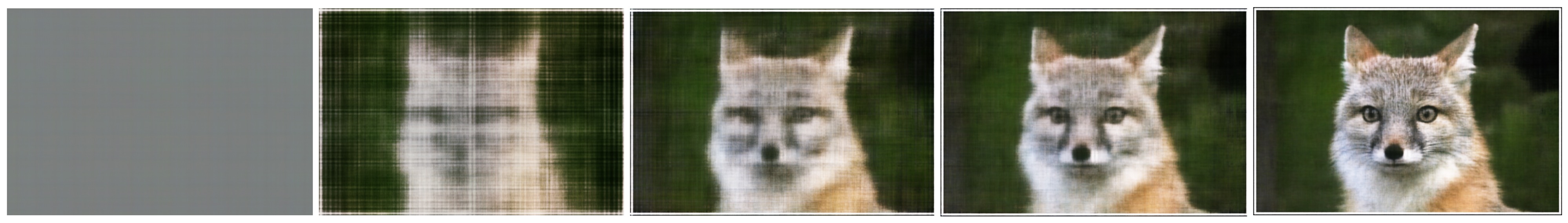
[Deliverables] As a reference, the above images show the process of optimizing the network to fit on this image.

• Report your model architecture including number of layers, width, and learning rate. Feel free to add other details you think are important. Tip: first implement the architecture shown above and see how your model performs to establish it works decently well. Then change the parameters as you deem best fit.
• Show training progression (images at different iterations, similar to the above reference) on both the provided test image and one of your own images.
• Show final results for 2 choices of max positional encoding frequency and 2 choices of width (a 2x2 grid of results). Try very low values for these hyperparameters to see how it affects the outputs.
• Show the PSNR curve for training on one image of your choice. Indicate the hyperparameters used for this run.

Part 2: Fit a Neural Radiance Field from Multi-view Images

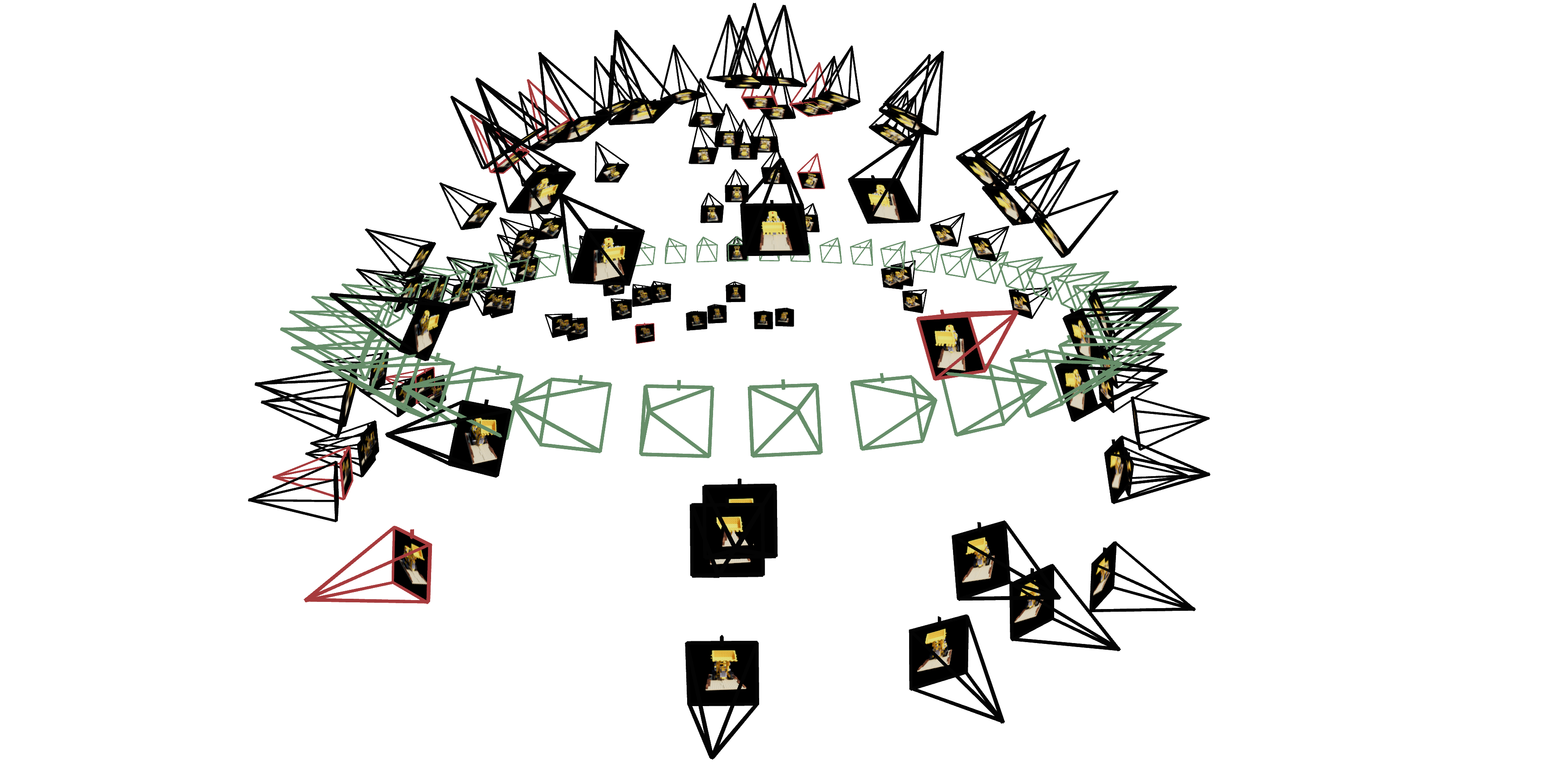
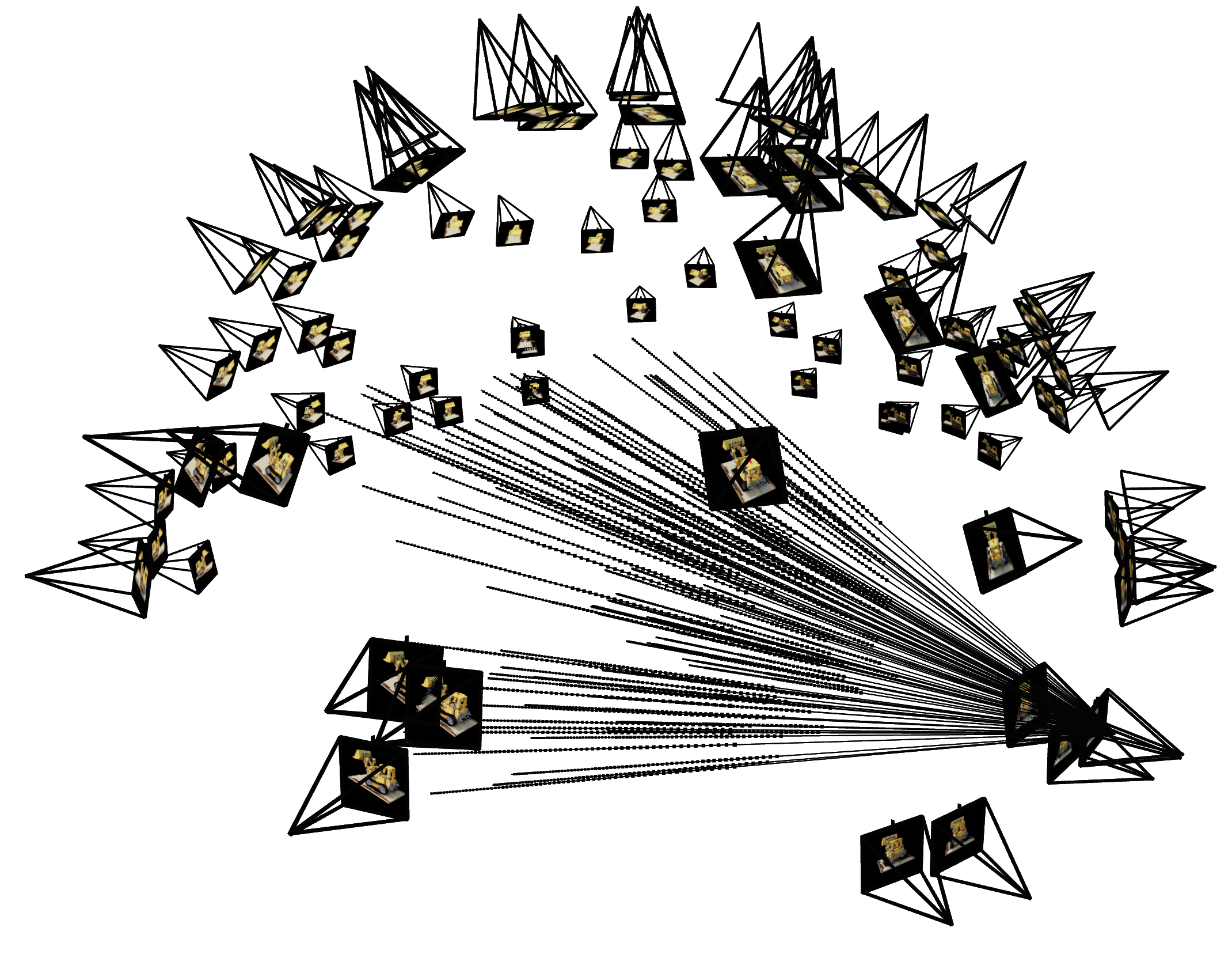
Now that we are familiar with using a neural field to represent a image, we can proceed to a more interesting task that using a neural radiance field to represent a 3D space, through inverse rendering from multi-view calibrated images. For this part we are going to use the Lego scene from the original NeRF paper, but with lower resolution images (200 x 200) and preprocessed cameras (downloaded from here). The figure on its right shows a plot of all the cameras, including training cameras in black, validation cameras in red, and test cameras in green.

The code found here can be used to parse the data.

---

Part 2.1: Create Rays from Cameras (implemented for you)

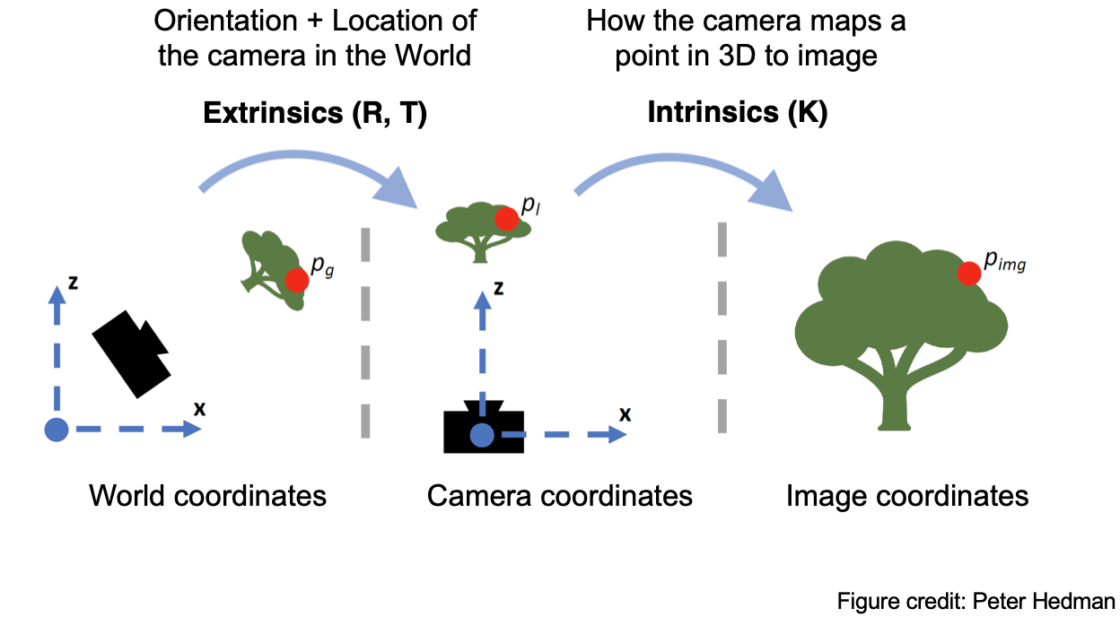
The following are the 3 main ‘coordinate system conversions’ you’ll be working with. They are already implemented for you in dataset_3d.py but are explained below for your perusal.

Camera to World Coordinate Conversion. Pre-computed and loaded from the dataset via load_data() in dataset_3d.py

The transformation between the world space \(\mathbf{X_w} = (x_w, y_w, z_w)\) and the camera space \(\mathbf{X_c} = (x_c, y_c, z_c)\) can be defined as a rotation matrix \(\mathbf{R}_{3 \times 3}\) and a translation vector \(\mathbf{t}\): \(\begin{bmatrix} x_c \\ y_c \\ z_c \\ 1 \end{bmatrix} = \begin{bmatrix} \mathbf{R}_{3\times3} & \mathbf{t} \\ \mathbf{0}_{1\times3} & 1 \end{bmatrix} \begin{bmatrix} x_w \\ y_w \\ z_w \\ 1 \end{bmatrix}\) in which \(\begin{bmatrix} \mathbf{R}_{3\times3} & \mathbf{t} \\ \mathbf{0}_{1\times3} & 1 \end{bmatrix}\) is called world-to-camera (w2c) transformation matrix, or extrinsic matrix. The inverse of it is called camera-to-world (c2w) transformation matrix.

Pixel to Camera Coordinate Conversion. Implemented for you via pixel_to_camera() in dataset_3d.py

Consider a pinhole camera with focal length \((f_x, f_y)\) and principal point \((o_x = \text{image_width} / 2, o_y = \text{image_height} / 2)\), its intrinsic matrix \(\mathbf{K}\) is defined as: \(\mathbf{K} = \begin{bmatrix} f_x & 0 & o_x \\ 0 & f_y & o_y \\ 0 & 0 & 1 \end{bmatrix}\) which can be used to project a 3D point \((x_c, y_c, z_c)\) in the camera coordinate system to a 2D location \((u, v)\) in pixel coordinate system : \(s \begin{bmatrix} u \\ v \\ 1 \end{bmatrix} = \mathbf{K} \begin{bmatrix} x_c \\ y_c \\ z_c \end{bmatrix}\) in which \(s=z_c\) is the depth of this point along the optical axis.

Pixel to Ray. Implemented for you via pixels_to_rays() in dataset_3d.py

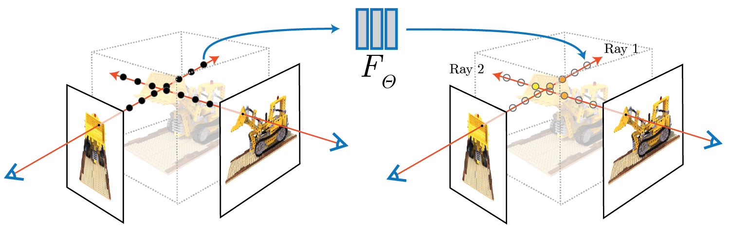
A ray can be defined by an origin vector \(\mathbf{r}_o \in \mathbb{R}^3\) and a direction vector \(\mathbf{r}_d \in \mathbb{R}^3\). In the case of a pinhole camera, we want to know the \(\{\mathbf{r}_o, \mathbf{r}_d\}\) for every pixel \((u, v)\). The origin \(\mathbf{r}_o\) of those rays is easy to get because it is just the location of the camera in world coordinates. For a camera-to-world (c2w) transformation matrix \(\begin{bmatrix} \mathbf{R}_{3\times3} & \mathbf{t} \\ \mathbf{0}_{1\times3} & 1 \end{bmatrix}\), the camera origin is simply the translation component: \(\mathbf{r}_o = \mathbf{t}\) To calculate the ray direction for pixel \((u, v)\), we can simply choose a point along this ray with depth equal to 1 (\(s=1\)) and find its coordinate in world space \(\mathbf{X_w} = (x_w, y_w, z_w)\) using your previously implemented functions. Then the normalized ray direction can be computed by: \(\mathbf{r}_d = \frac{\mathbf{X_w} - \mathbf{r}_o}{\|\mathbf{X_w} - \mathbf{r}_o\|_2}\)

---

Part 2.2: Sampling

[Impl: Sampling Rays from Images]

In Part 1 we did random sampling on a single image to get the color and (u, v) coordinates of each pixel.

Here we build on top of that and for each set of pixel coordinates determine the ray origin and direction associated by using the camera intrinsics and extrinsics. Make sure to account for the offset from image coordinate to pixel center (this can be done simply by adding .5 to your UV pixel coordinate grid)!

At this point, we’re operating on multiple images at once and have two options of sampling rays—e.g., N rays—at every trainin giteration:

1. Sample M images, and then sample N // M rays from every image.
2. Flatten all pixels from all images and do a global sampling once to get N rays from all images.

You can choose whichever way you do ray sampling.

Note: this corresponds to implementing RaysData.sample_rays() in dataset_3d.py. You will have to do all preprocessing in the RaysData.__init__() function. You also need to have implemented images_to_rays() to use it in sample_rays(). Regarding images_to_rays(): you can first implement image_to_rays() and then call it in a for loop for images_to_rays(), or you can directly implement a vectorized images_to_rays() version. The decision is yours!

[Impl: Sampling Points along Rays.]

Now that we can sample rays (origin + direction), we also need to discretize each ray into samples along the ray that live in the 3D space.

The simplest way is to uniformly create some samples along the ray (using torch.arange(num_samples_along_ray)). For the lego scene that we have, we can set near=2.0 and far=6.0. The actual 3D coordinates can be acquired by $\mathbf{x} = \mathbf{r}_o + t \mathbf{r}_d$.

Note: this would use a fixed set of 3D points, which could potentially lead to overfitting when we train the NeRF later on. Therefore, we want to introduce some small perturbation to the points only during training, so that every location along the ray would be touched upon during training. this can be achieved by something like t = t + (np.random.rand(t.shape) * t_width) where t is set to be the start of each interval. This corresponds to the perturb boolean argument passed into sample_along_rays() in rendering.py.

We recommend to set n_samples to 32 until your NeRF pipeline training works (loss goes down) and then changing to 64. You can also potentially keep it 32 the entire time.

Note: this corresponds to implementing sample_along_rays() in rendering.py.

---

Part 2.3: Putting the Dataloading All Together

Similar to Part 1, you would need to write a dataloader that randomly sample pixels from multiview images. What is different with Part 1, is that now you need to convert the pixel coordinates into rays in your dataloader, and return ray origin, ray direction and pixel colors from your dataloader.

[Impl: Fully working RayData and sample_along_rays().]

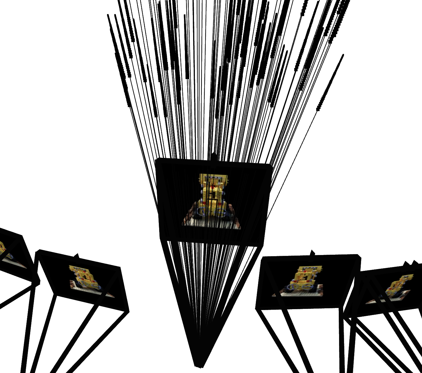
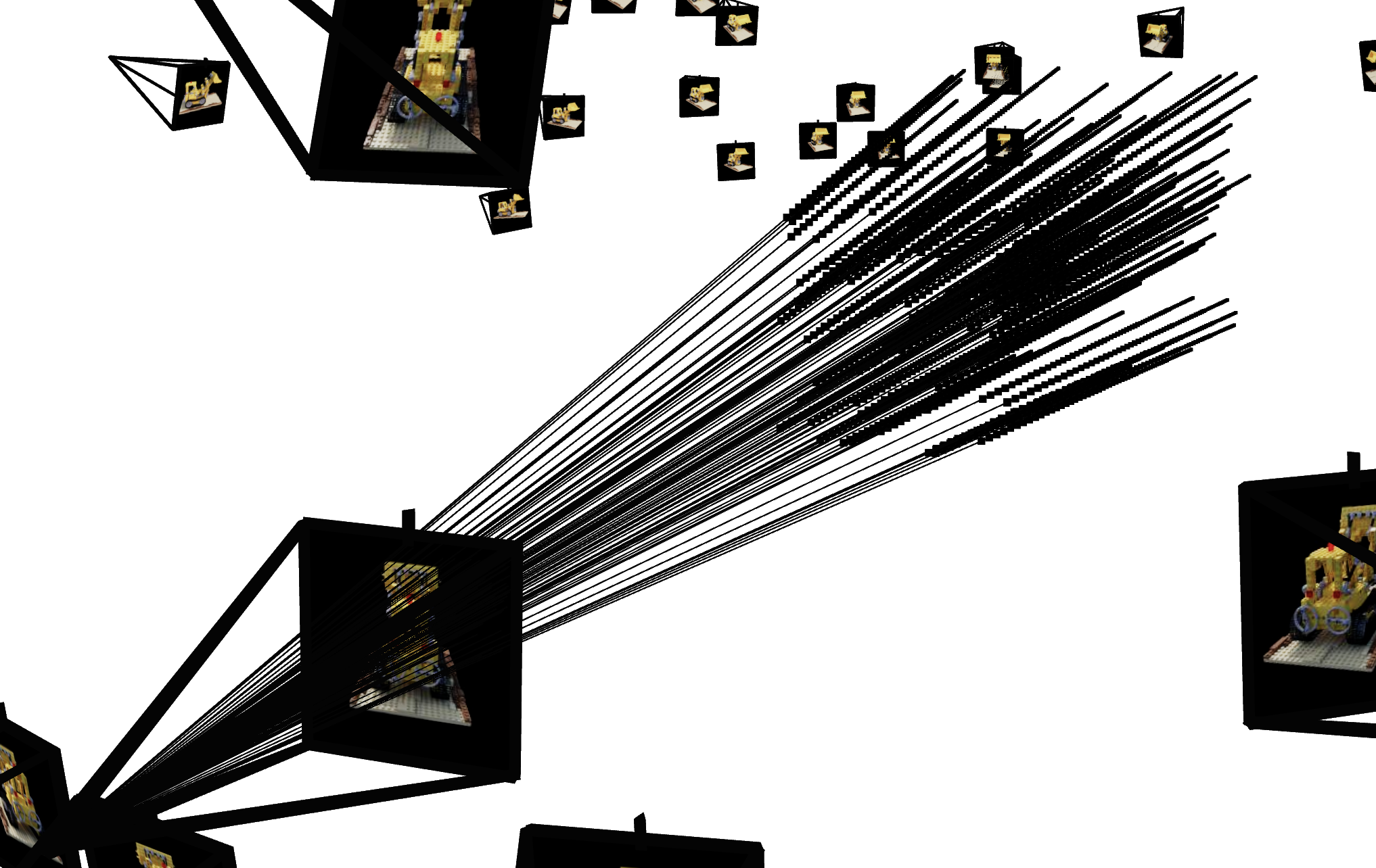
To verify if you have by far implement everything correctly, we here provide some Viser visualization code here to plot the cameras, rays, and samples in 3D.

We additionally recommend you try this code with rays sampled only from one camera so you can make sure that all the rays stay within the camera frustum and eliminating the possibility of other smaller harder to catch bugs. You can toggle this once you’ve launched the viser server and adjusting the number of cameras.

Note: you will have to provide these visualization results in your submission.

---

Part 2.4: Neural Radiance Field

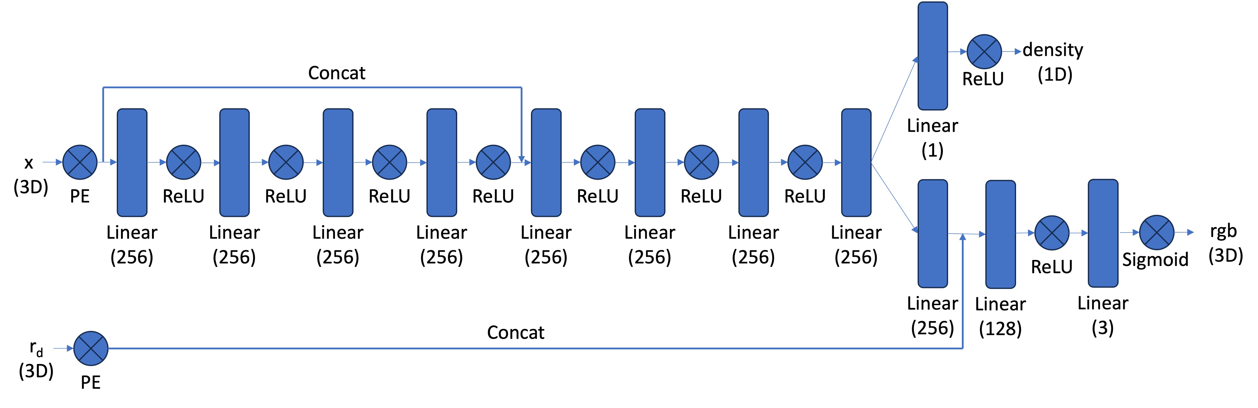
[Impl: Network] After having samples in 3D, we want to use the network to predict the density and color for those samples in 3D. So you would create a MLP that is similar to Part 1, but with three changes:

• Input is now 3D world coordinates instead of 2D pixel coordinates, along side a 3D vector as the ray direction. And we are going to output not only the color, but also the density for the 3D points. In the radiance field, the color of each point depends on the view direction, so we are going to use the view direction as the condition when we predict colors. Note we use Sigmoid to constrain the output color within range (0, 1), and use ReLU to constrain the output density to be positive. The ray direction also needs to be encoded by positional encoding (PE) but can use less frequency (e.g., L=4) than the cooridnate PE (e.g., L=10).
• Make the MLP deeper. We are now doing a more challenging task of optimizing a 3D representation instead of 2D. So we need a more powerful network.
• Inject the input (after PE) to the middle of your MLP through concatenation. It’s a general trick for deep neural network, that is helpful for it to not forgetting about the input.

Below is a structure of the network that you can start with:

---

Part 2.5: Volume Rendering

The core volume rendering equation is as follows:

\[C(\mathbf{r})=\int_{t_n}^{t_f} T(t) \sigma(\mathbf{r}(t)) \mathbf{c}(\mathbf{r}(t), \mathbf{d}) dt, \text{ where } T(t)=\exp \left(-\int_{t_n}^t \sigma(\mathbf{r}(s)) ds\right)\]

This fundamentally means that at every small step \(dt\) along the ray, we add the contribution of that small interval \([t, t + dt]\) to that final color, and we do the infinitely many additions of these infinitesimally small intervals with an integral.

The discrete approximation (thus tractable to compute) of this equation can be stated as the following: \(\hat{C}(\mathbf{r})=\sum_{i=1}^N T_i\left(1-\exp \left(-\sigma_i \delta_i\right)\right) \mathbf{c}_i, \text { where } T_i=\exp \left(-\sum_{j=1}^{i-1} \sigma_j \delta_j\right)\) where \(\mathbf{c}_i\) is the color obtained from our network at sample location \(i\), \(T_i\) is the probability of a ray not terminating before sample location \(i\), and \(1 - e^{-\sigma_i \delta_i}\) is the probability of terminating at sample location \(i\).

This is already implemented for you in rendering.py.

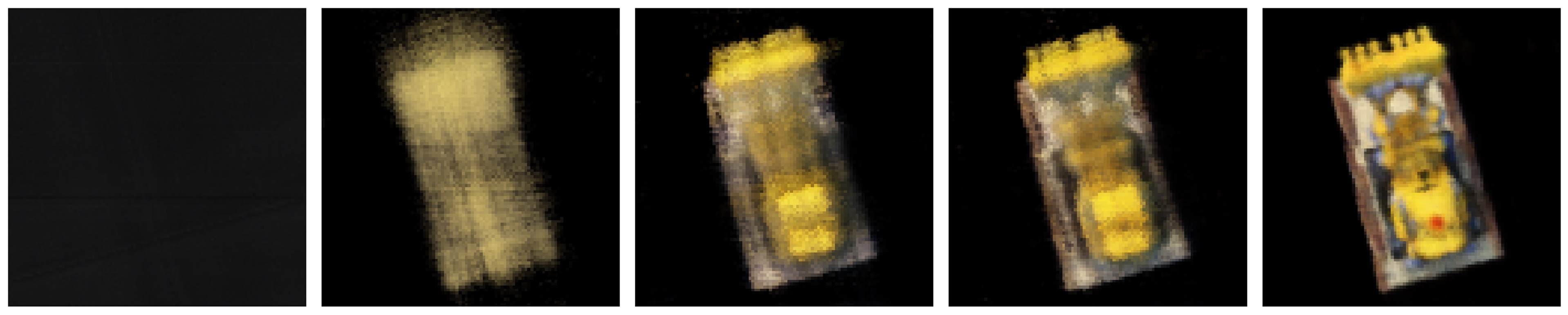
[Deliverables] As a reference, the images below show the process of optimizing the network to fit on our lego multi-view images from a novel view. The staff solution reaches above 23 PSNR with 1000 gradient steps and a batchsize of 10K rays per gradent step. The staff solution uses an Adam optimizer with a learning rate of 5e-4. For guaranteed full credit, achieve 23 PSNR for any number of iterations.

• Include a brief description of how you implement each part.
• Report the visualization of the rays and samples you draw at a single training step (along with the cameras), similar to the plot we show above. Plot up to 100 rays to make it less crowded.
• Visualize the training process by plotting the predicted images across iterations, similar to the above reference, as well as the PSNR curve on the validation set (6 images).
• After you train the network, you can use it to render a novel view image of the lego from arbitrary camera extrinsic. Show a spherical rendering of the lego video using the provided cameras extrinsics (c2ws_test in the npz file). You should get a result like this:

After 1000 training iterations

After 5000 training iterations

Part 3: Training a NeRF with Your Own Data (10 pt. extra credit)

We will now create a NeRF with our own real-world data. Our aim is to create an .npz file that contains the data in the same format as the Lego dataset, with some modifications.

To get camera poses, we will use COLMAP, a very popular SfM and MVS pipeline.

Part 3.1 Capturing a Scene

For best results, we want:

• Our scene to be object-centric, meaning we capture an object (such as a toy) and not a landscape or planar surface.
  • Note: we don’t want our object to be too small, otherwise there wouldn’t be much parallax between views and COLMAP will struggle.
• Our object to be textured, since COLMAP works best with textured scenes.
• Our object to be centered in each image. Later, we’ll want to center-crop each image and want to keep the object in the image.
• Enough views of the object to be able to
  1. Get good pose estimations.
  2. Train an accurate NeRF.
     • Even if we pass in, say, 100 views into COLMAP, COLMAP may only find poses for 20 of them, meaning we’d only have 20 views to train on. Ideally we have ~60 images to train the NeRF on like in the Lego dataset. You’ll have to recapture the scene until COLMAP returns enough views with decent poses.
• The first image of the scene should be at the same height of the object and pointing at it directly. This will be used to determine the origin of the scene and will avoid a lot of headache when we create the gif later.

Part 3.2 Running COLMAP on the Captured Scene

To create this custom dataset, you’re welcome to use the provided code in this Google Colab notebook. At a high level, we need to:

1. Capture images of the scene by one of the following methods:
   1. Capturing individual photos (taking care to not change camera parameters between shots)
   2. Recording a video around the object and subsampling frames to get enough views. You can play around with different subsampling rates to get enough views. Course staff used this method.
2. Run COLMAP on the captured frames in step 1. Importantly:
   1. COLMAP will work better on higher resolution images. That said, COLMAP is expensive to run and you will likely need to downsample your images for faster processing. Note: this means that the c2w matrices and focal lengths returned by COLMAP will be scaled down from the original scale of the captured scene. Later we will have to scale them back up to the original scale.
   2. COLMAP may not give enough views (and therefore not enough training data) the first time around. You’ll have to adjust the number of images you’re passing into COLMAP, the resolution of these images that COLMAP uses, and may even have to recapture scenes (taking longer recordings or choosing scenes with more textures and parallax) until COLMAP returns decent enough views.
   3. For consistency, we scale the c2w matrices and focal lengths returned by COLMAP back to the original scale of the captured scene.
3. Create the .npz file for our custom dataset. This means center cropping the images and downsampling to a resolution that is suitable for training the NeRF (in our case, 200x200 like in the Lego dataset). This means we also have to adjust the c2w matrices and focal lengths to reflect this change. Important: this also means undistorting the images using something like cv2.undistort(img, camera_matrix, dist_coeffs) since NeRF assumes a perfect pinhole camera model without distortion.
   • Note: the deliverable doesn’t require test poses, and therefore we save all our posed images in the .npz file as images_train, c2ws_train, and focal. You are welcome to create train, validation, and test splits from this data as you see fit. For debugging, we recommend that you put aside ~5 images as a validation set and render them throughout training, like we did in part 2.
4. Passing in this newly created .npz into part 3.3 below.

[Impl] Run COLMAP on the captured scene and save the camera poses and intrinsics to a .npz file. Use your pipeline from part 2 to train this NeRF.

Part 3.3 Training the NeRF

Use your code from part 2, swapping out the Lego .npz for your own and swapping hyperparameters as needed.

Helpful Tips / Common Mistakes:

• For the lego dataset, our near and far parameters were set to 2.0 and 6.0 respectively. You will likely have to adjust these for the real data you collect. These parameters represent the minimum and maximum distance away from the camera’s sensor that we start and stop sampling. For our example we found that near = 2.0 and far = 6.0 worked well, but you will likely have to do some experimenting to find values that work for you. For example, others scenes required near = 0.02 and far = 0.5.
• You might want to increase the number of samples along your rays for your real data. This will take longer to train, but can improve visual quality of your NeRF. For our implementation we first trained with 32 samples in order to ensure that there are no issues or bugs in other parts of our code and then increased to 64 samples per ray to get our final result.
• If training is taking an unreasonable amount of time, your image resolution may be the issue. Attempting to train with too large of images may take a long time. If you resize your images you need to ensure that your intrinsics matrix reflects this change either by resizing before doing calibration or adjusting the intrinsics matrix after recovering it.

[Impl] Train a NeRF on your chosen object dataset collected in part 0. Make sure to save the training loss over iterations as well as to generate intermediate renders for the deliverables.

Part 3.4 Visualizing the Output

For debugging purposes, look at the intermediate renders you created in part 3.3.

For the deliverable, create a gif where the camera is orbiting the object and showing the rendered views. We encourage you to use the provided code here to help you visualize the scene. A couple of helpful tips:

• Your axes may be flipped compared to the provided code. You may need to play around with different axes of rotation.
• Your scene scale will likely be different for each scene you capture. You will likely need to play around with the near and far parameters and the camera starting position to get the best results.
  • For example, if it looks like your camera is only rotating around an axis but not translating around an object, you are likely too close to the scene origin and need to move back.

[Deliverables] Create a gif of a camera circling the object showing novel views and discuss any code or hyperparameter changes you had to make. Include a plot of the training loss as well as some intermediate renders of the scene while it is training.

Sample training image

Orbit render after training

Bells & Whistles (Optional)

• Render the depths map video for the Lego scene. Instead of compositing per-point colors to the pixel color in the volume rendering, we can also composite per-point depths to the pixel depth. (See the reference video below)

The following are optional explorations for any students interested in going deeper with NeRF.

• Better (more efficient) sampling: Implement course-to-fine PDF resampling as described in the original NeRF paper.
• Better NeRF representations: Replace MLP with something more advanced to make it faster. (e.g. TensoRF or Instant-NGP). For this part it is ok to borrow some code from existing implementations (mark reference!) to your code base and see how it affect your NeRF optimization.
• Improve PSNR to 30+: Aside from better sampling, better NeRF representations, try other things you can think of to improve the quality of the images to get 30+ db in PSNR.
• Render the Lego video with a different background color than black. You would need to revisit the volume rendering equation to see where you should inject the background color.
• Implement scene contraction for large scenes as specified in Mip-NeRF 360. This allows NeRF to handle unbounded scenes by contracting distant points into a bounded space.
• Use nerfstudio to make a cool video!

Deliverables Checklist

Make sure your submission (website + pdf) includes all of the following:

Part 1: Fit a Neural Field to a 2D Image

• Model architecture report (number of layers, width, learning rate, and other important details)
• Training progression visualization on both the provided test image and one of your own images
• Final results for 2 choices of max positional encoding frequency and 2 choices of width (2x2 grid)
• PSNR curve for training on one image of your choice

Part 2: Fit a Neural Radiance Field from Multi-view Images

• Brief description of how you implemented each part
• Visualization of rays and samples with cameras (up to 100 rays)
• Training progression visualization with predicted images across iterations
• PSNR curve on the validation set
• Spherical rendering video of the Lego using provided test cameras

Part 3: Training with Your Own Data (10 pt. extra credit)

We may do a class vote later for best NeRF!

• GIF of camera circling your object showing novel views
• Discussion of code or hyperparameter changes you made
• Plot of training loss over iterations
• Intermediate renders of the scene during training

Bells & Whistles (optional)

• Depth map video for the Lego scene
• Any additional exploration you do!

Acknowledgements

This assignment is based on Angjoo Kanazawa and Alyosha Efros’s version at Berkeley.