Homework 2
COMS4732: Computer Vision 2

AUTOMATIC FEATURE MATCHING ACROSS IMAGES
Due Date: Thursday, February 19 at 11:59 PM EST

Background

This assignment will involve creating a system for automatically detecting corresponding features in 2 images.

We will loosely follow the paper “Multi-Image Matching using Multi-Scale Oriented Patches” by Brown et al. but with several simplifications. Read the paper first and make sure you understand it at a high level, then we will implement parts of the algorithm. Note: we will implement a simpler version of Adaptive Non-Maximal Suppression (ANMS) instead of the version described in the paper - no worries if you don’t understand it fully.

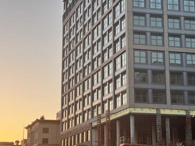
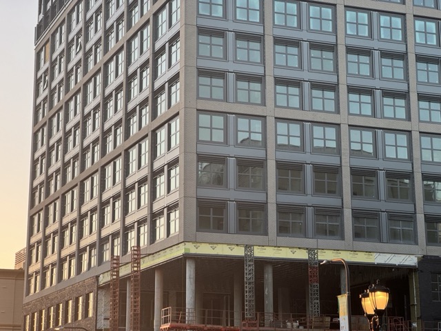
Step 0: Taking photos (0 points, required)

Take your 2 photos as you would a panoramic, remembering to keep your camera level, only rotating your camera but not translating it. Additionally, make sure to lock the exposure and focus of your camera such that they don’t change between the two photos.

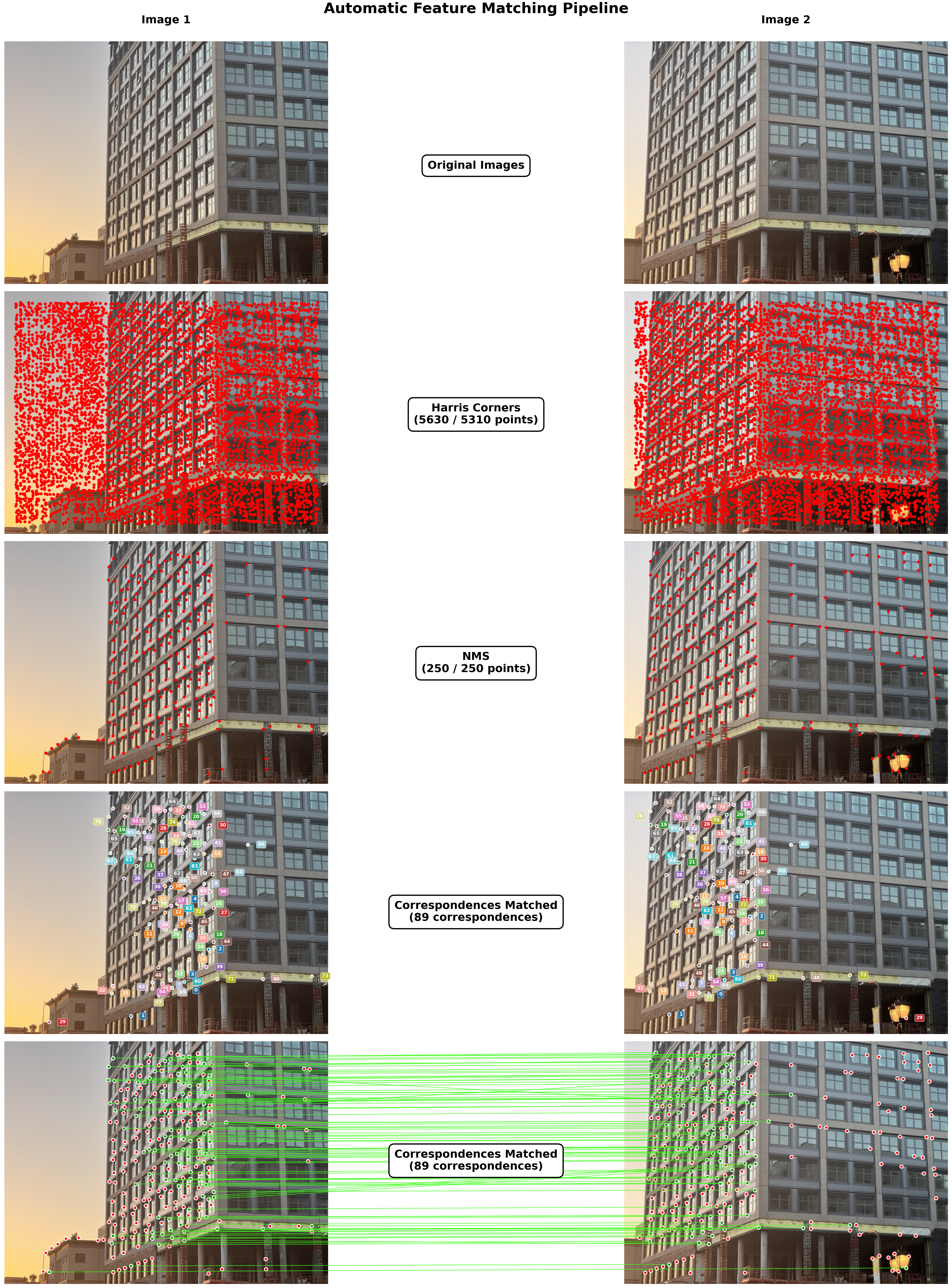
Step 1: Harris Corner Detection (5 points)

Start with Harris Interest Point Detector (Section 2). We won’t worry about multi-scale – just do a single scale. Also, don’t worry about sub-pixel accuracy. Re-implementing Harris is a thankless task – so you can use our sample code: harris.py.

Step 1 Deliverable

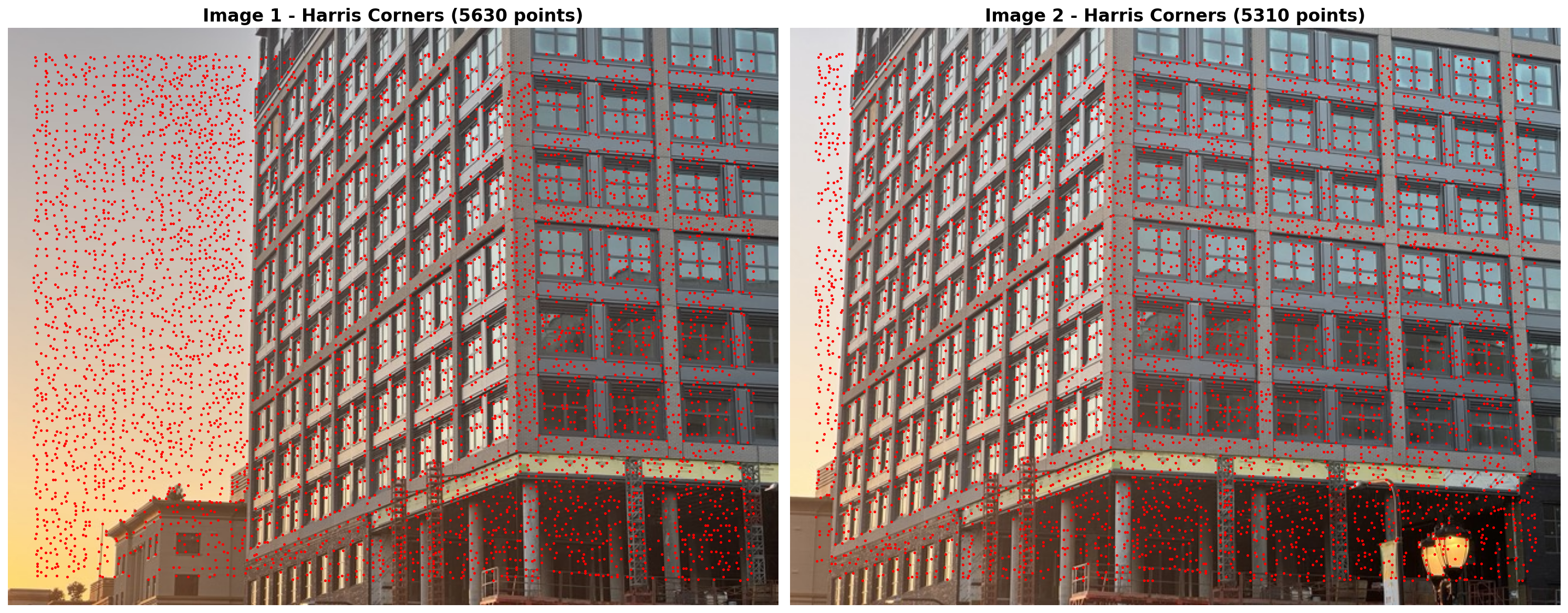
Deliverables: Show your 2 images, as-is, side-by-side. Also, show detected corners overlaid on your set of images side-by-side.

Step 2: Non-Maximal Suppression (NMS) (15 points)

Instead of the Adaptive Non-Maximal Suppression (ANMS) described in the paper, we will implement a simpler version of Non-Maximal Suppression (NMS) where we simply discard all corners that are not the local maximum in a window with our choice of size. Report the window size you used.

Step 2 Deliverable

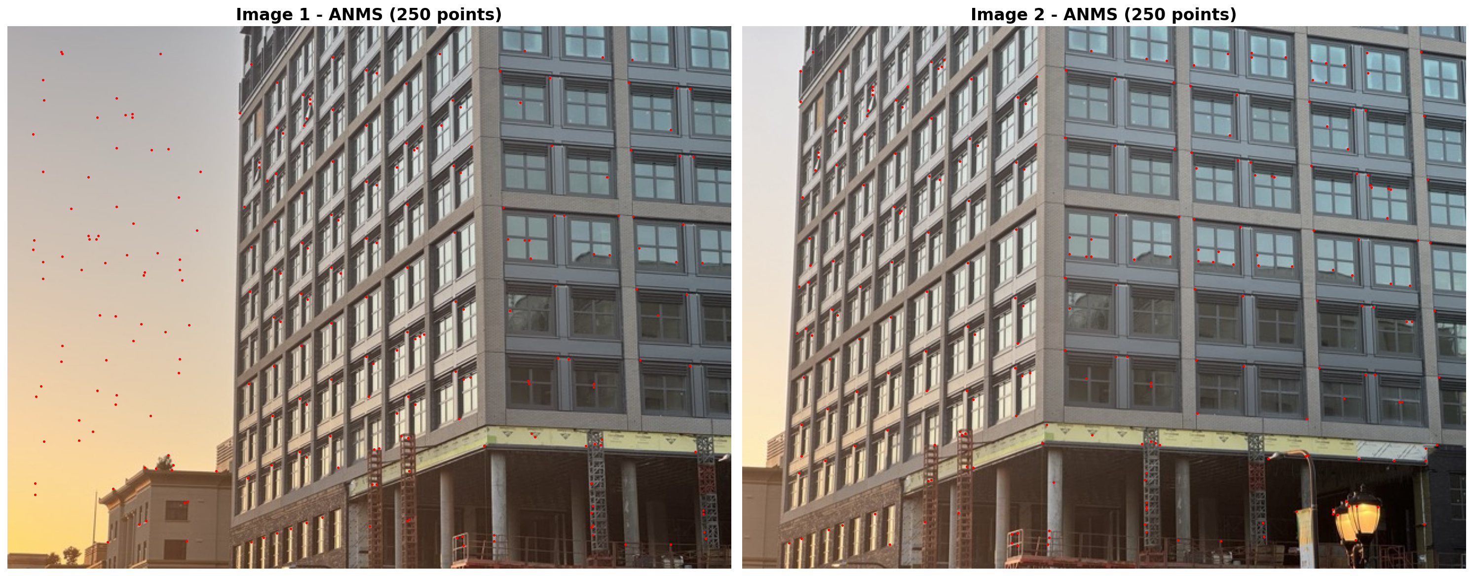
Deliverables: Show chosen corners overlaid on your set of images side-by-side after applying NMS.

Step 3: Feature Descriptor Extraction (5 points)

Implement Feature Descriptor extraction (Section 4 of the paper). Don’t worry about rotation-invariance – just extract axis-aligned 8x8 patches. The paper describes this in a confusing way, so here’s a clarification: we just want to take a 40x40 patch around a corner and downsample it to 8x8. We turn on anti_aliasing=True, which internally applies a Gaussian blur before downsampling, via something like downscaled_window = resize(window, (8, 8), anti_aliasing=True). This way, we have a nice blurred descriptor that doesn’t have any aliasing artifacts. Don’t forget to bias/gain-normalize the descriptors. Ignore the wavelet transform section.

Deliverables: deliverable is part of step 4

Step 4: Feature Matching (15 points)

Implement Feature Matching (Section 5 of the paper). That is, you will need to find pairs of features that look similar and are thus likely to be good matches. There are 2 approaches for this:

Nearest neighbor matching: Find the nearest neighbor for each feature in the other image and check if the distance is less than some threshold.
Lowe’s ratio test / NN distance ratio (NNDR):
- Threshold on the ratio between the first and the second nearest neighbors. Consult Figure 6b in the paper for picking the threshold. Ignore Section 6 of the paper.
- The idea here is that a good descriptor from img2 should be significantly better than the other img2 descriptor candidates while still being close to the img1 descriptor.

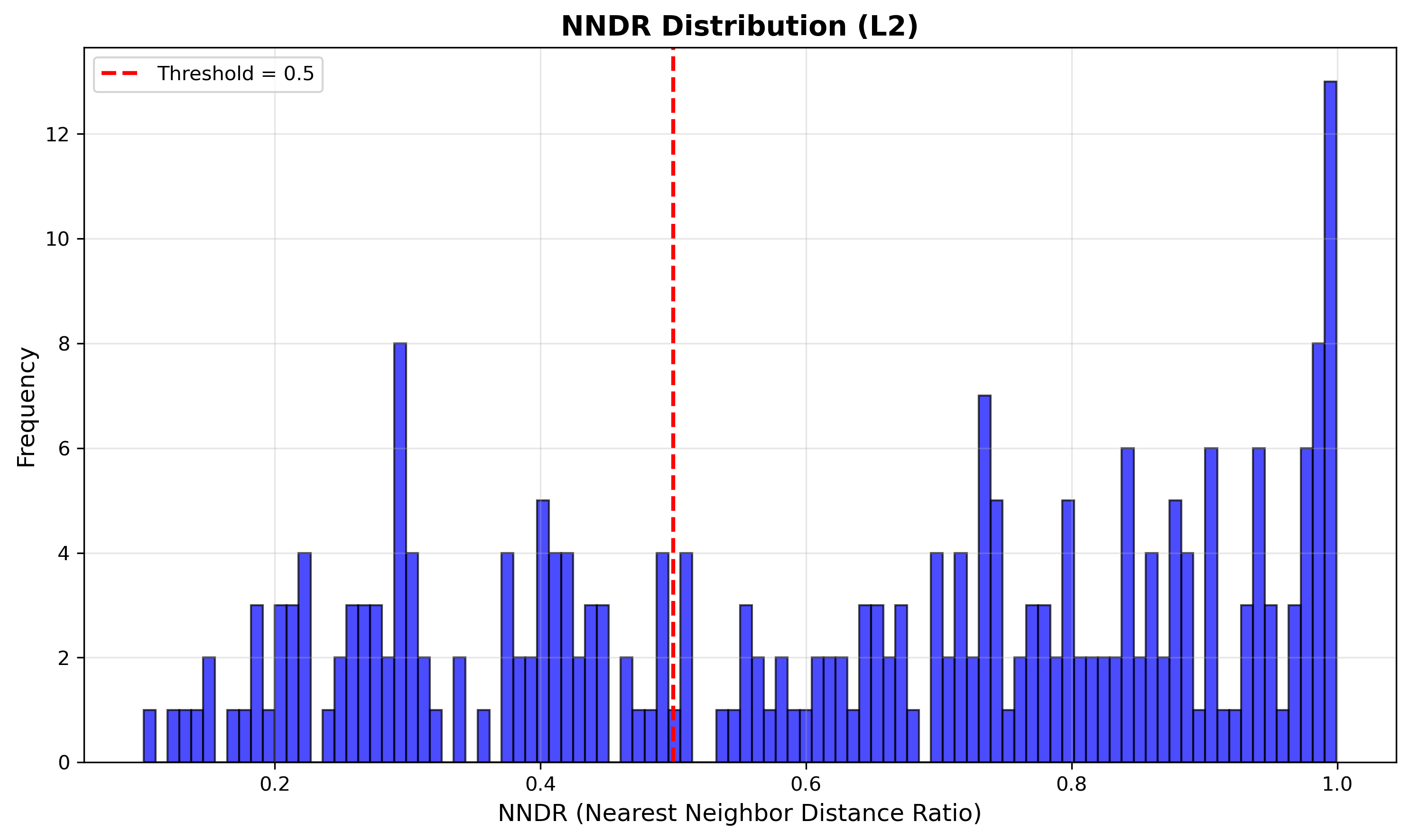
You will implement the latter: for your set of images, display the NNDR histogram and highlight the threshold you used.

Step 4.3 Deliverable

Deliverables:

Display the NNDR histogram and highlight the threshold you used. Also specify which similarity metric you used (e.g. SSD, NCC, etc.).
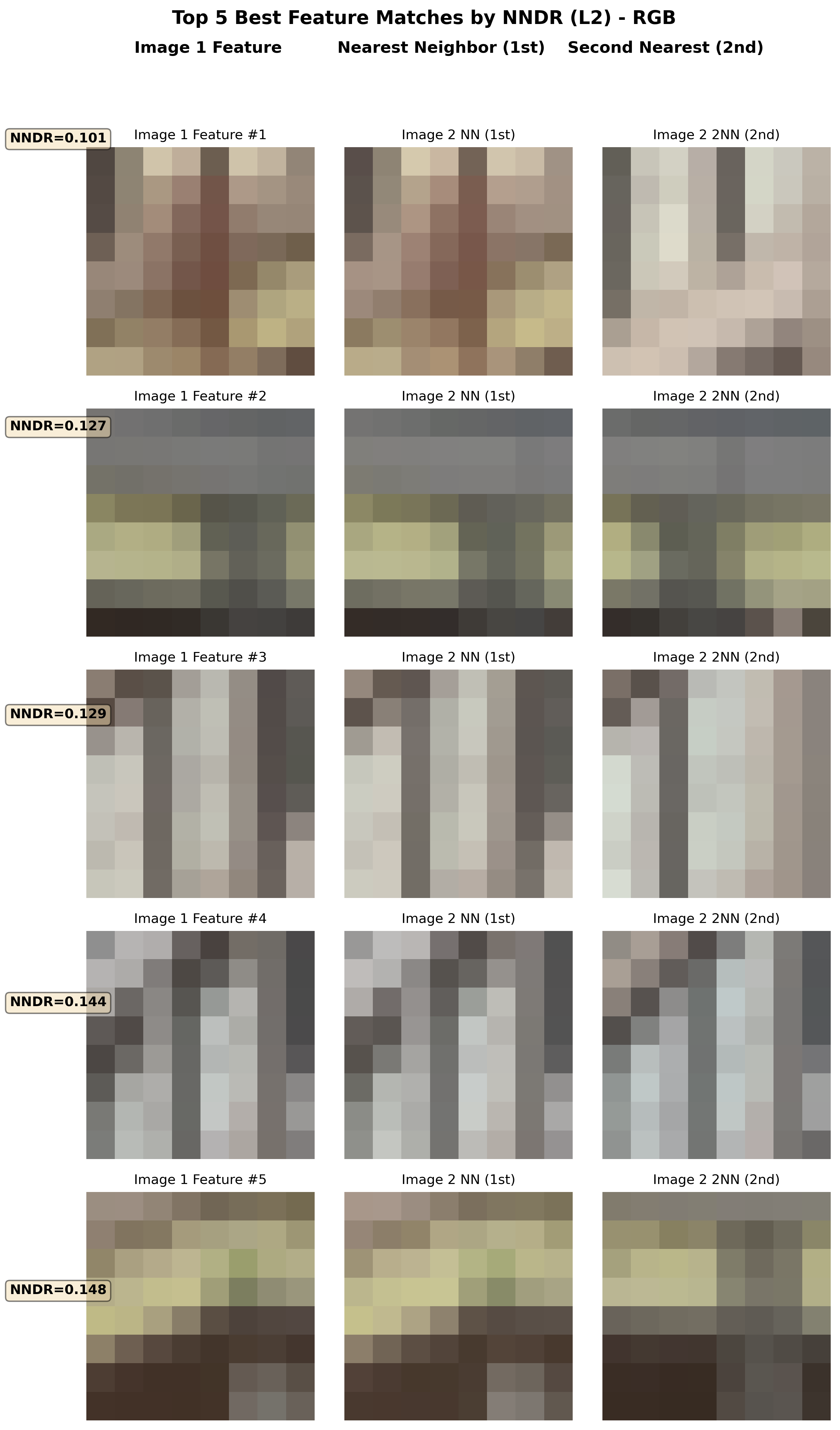
Visualize the 5 best feature matches between the 2 images (no worries if you don’t have 10 matches, just show as many as you can).
1. the first column should be the feature descriptor for img1’s feature.
2. the second column should be the 1NN feature descriptor from img2.
3. the third column should be the 2NN feature descriptor from img2.
Visualize the matches using one of the 2 options:
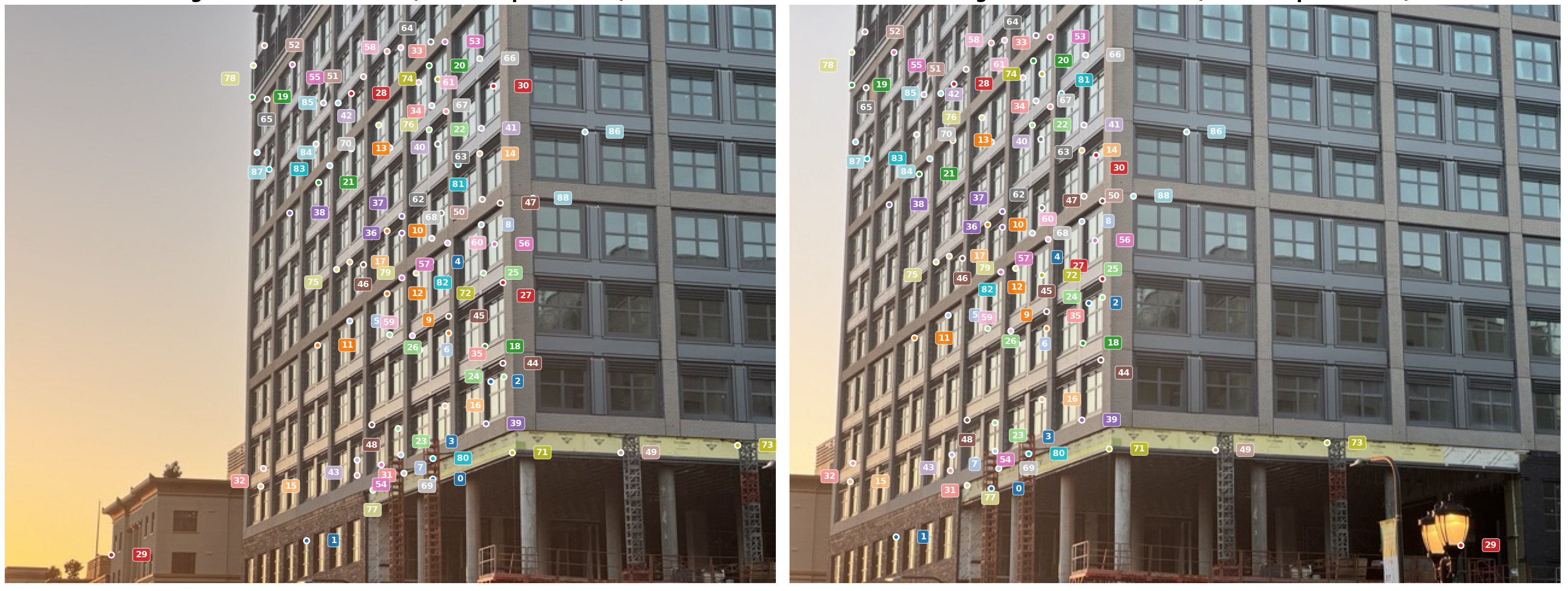
- Option 1: Color-code the matched features across both images and display them side-by-side. Also, put a number next to each feature to indicate the match index.
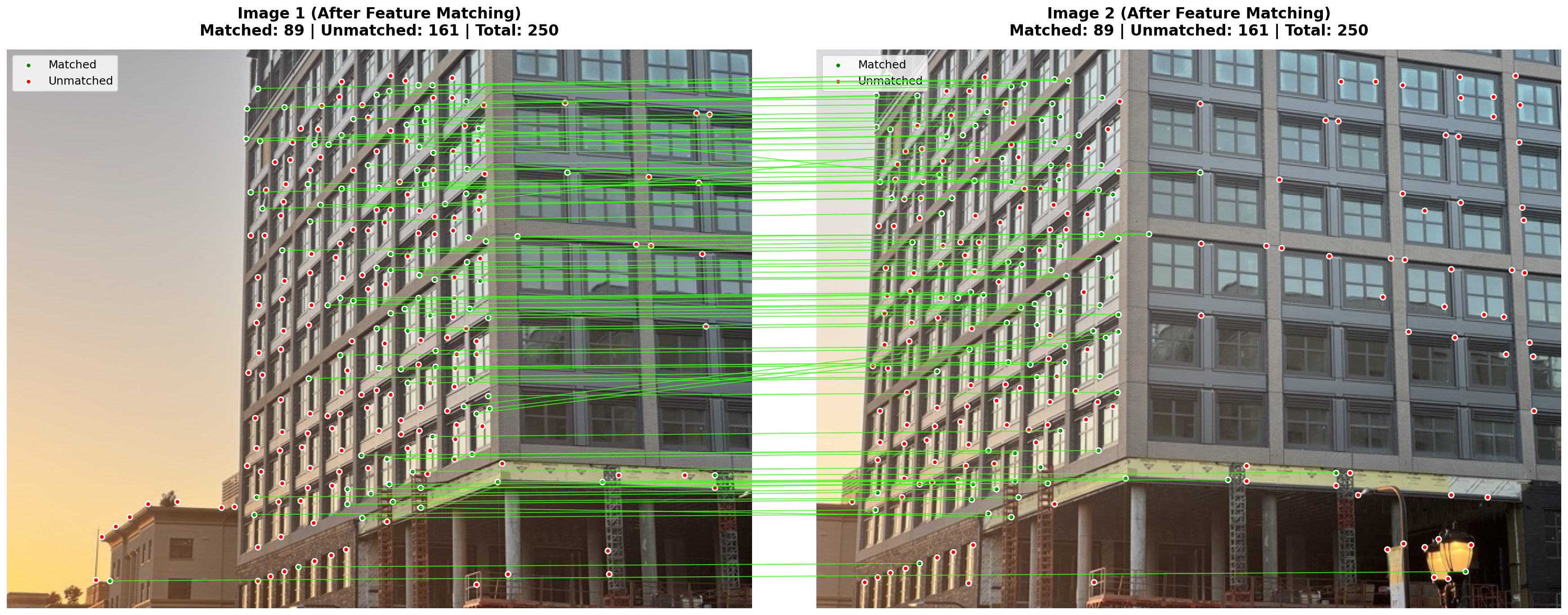
- Option 2: Draw green lines between matched features across both images side-by-side, and put red dots on the unmatched features.

Hint:

These matches aren’t supposed to be perfect. In the next HW (HW3), we use RANSAC to estimate the homography (geometry) that relates these two images. This is also known as “geometric validation” since we would only keep the matches that are consistent with the estimated homography/geometry.

Extra credit: Image Stitching/Panorama (10 points to be used on entire HW category in class)

From at least 2 images, create an image panorama by stitching them together. This means using RANSAC to estimate the homography that relates the images, then stitching them together by warping one image via the homography, performing inverse warping, then blending the images together. You are welcome to use any libraries you want to do this, but you must use the features you computed in the previous steps.

HW extra credit in this class will work as follows: you can get up to 10 points of extra credit for completing this part. This can go towards any points you miss on homeworks in this class (meaning all 5 assignments), but it cannot bring you past 100% in the HW category.

Bells & Whistles (Optional)

Adaptive Non-Maximal Suppression (ANMS): Implement Adaptive Non-Maximal Suppression (ANMS) as described in the paper.
RANSAC to estimate the homography: Implement RANSAC to estimate the homography as described in the paper. This will yield better feature matches since they will have been geometrically verified by finding all the inliers according to the homography.
Image Panorama: Create a panoramic image from the 2 images by stitching them together using the homography and blending the images together.
Rotation invariance: Add rotation invariance to the MOPS feature descriptors.
Support for 3+ images: Implement support for 3+ images by using the homography to stitch together more than 2 images.

Hints

You are strongly encouraged to use LLMs to implement any visualization code you wish. Past iterations of this assignment (pre LLMs) had to code these up themselves! Lucky for you, these LLMs are in your pocket now. You can only use LLMs for visualization code only.
If you would like to visually debug using the staff example, the images can be found here: img1.jpg and img2.jpg
You are encouraged to read the paper and discuss with other students what hyperparameters you used. Closer to the due date, staff may provide their own hyperparameters for the staff example.

Deliverables

You must submit results for 2 different scenes / pairs of images. The staff example images do not count.

Submit your code, input images, and html webpage (index.html and assets folder), README.md to Gradescope as a .zip file. File size limit is 100MB. This should contain 2 scenes with visualizations like the ones shown below (with at least 1 of the 2 feature matching visualizations chosen):