Homework 3
COMS4732: Computer Vision 2

SIMPLE STRUCTURE FROM MOTION
Due Date: Thursday, March 5 11:59PM ET

Starter code can be found here.

Collapse all

Overview

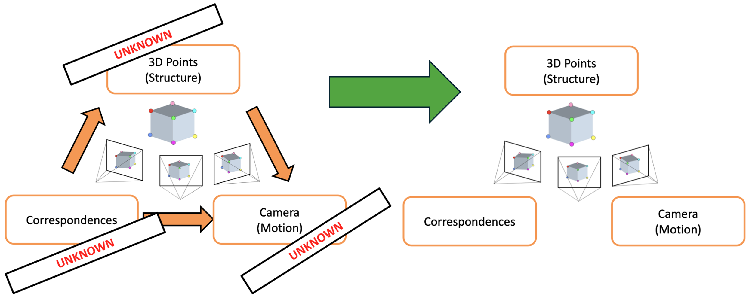
In this assignment, you’ll build components of a simple Structure from Motion (SfM) pipeline that estimates correspondences, camera position/motion, and 3D scene points from a pair of images. By the end of this assignment, you’ll be able to generate a sparse point cloud and visualize the rotation and translation that relates the 2 cameras.

You will use the staff-provided images (img1_1280x960.jpeg, img2_1280x960.jpeg).

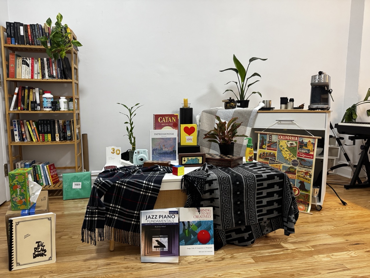
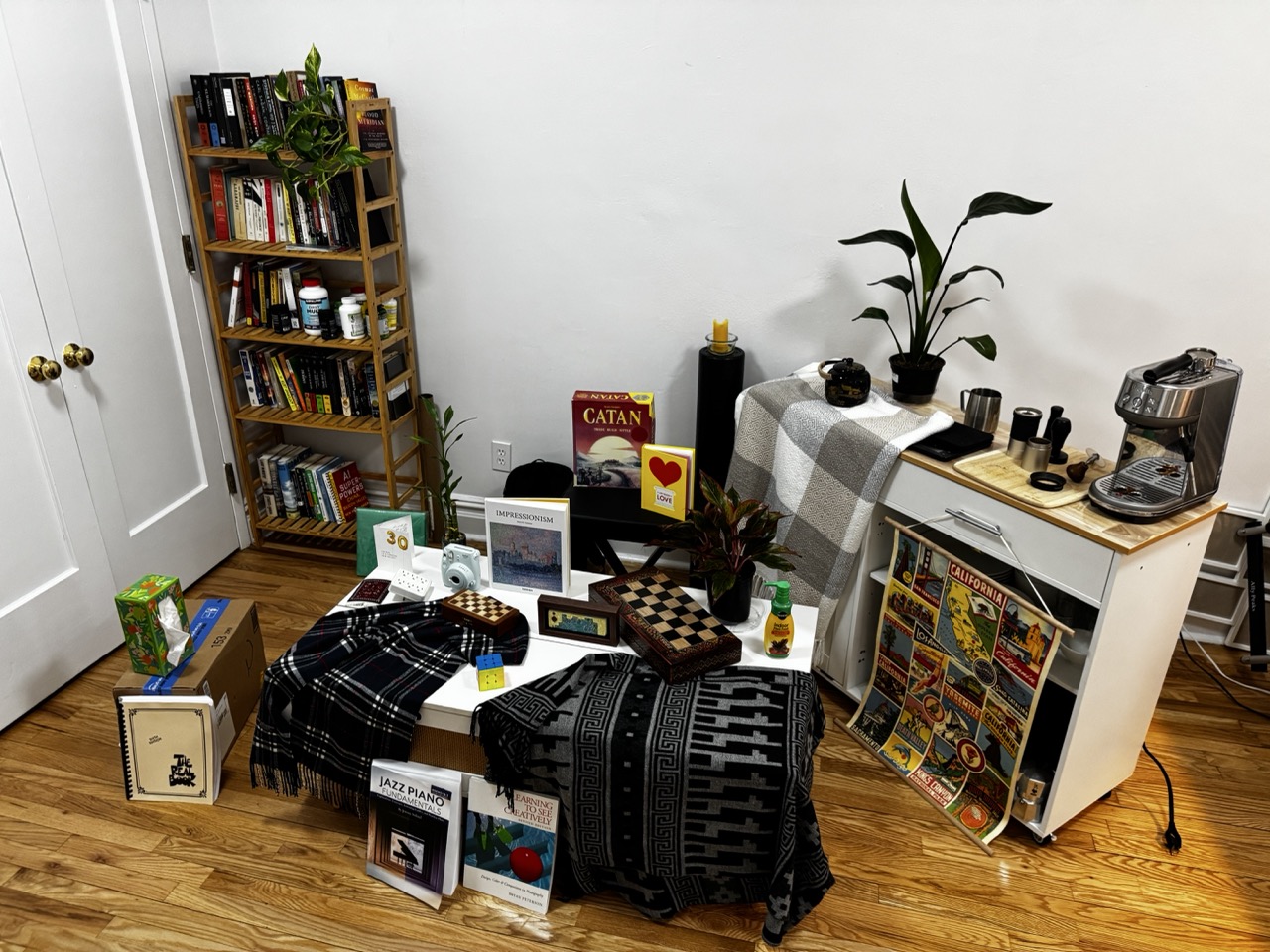
Ryan's living room out of equilibrium

If you’re interested in why this setup is the way it is and how to optimally capture your own scene, see instructions below on capturing your own scene.

Step 1: Computing Camera Intrinsics (15 points)

This assignment involves stereo on calibrated cameras, meaning with known camera intrinsics. Note that the more general version of SfM uses uncalibrated cameras–meaning we don’t know the intrinsics–though we leave this as an exercise to the reader.

Step 1 of this pipeline involves computing the intrinsic matrix $K$ for the camera associated with the images used:

\[K = \begin{bmatrix} f_\text{px} & 0 & c_x \\ 0 & f_\text{px} & c_y \\ 0 & 0 & 1 \end{bmatrix}, \qquad c_x = \frac{W_\text{px}}{2},\quad c_y = \frac{H_\text{px}}{2}\]

where $f_\text{px}$ is the camera focal length in terms of number of pixels, $W_\text{px}$ is the number of horizontal pixels and $H_\text{px}$ is the number of vertical pixels, and $(c_x, c_y)$ is the principal point at the center of the image plane (i.e., center of image).

For the staff-provided images (captured with an iPhone 15 Pro on the main camera / 1x zoom):

• physical focal length: $f_\text{mm} = 6.765$mm
• physical camera sensor height: $h_\text{mm} = 7.318$mm
• physical camera sensor width: $w_\text{mm} = 9.757$mm

From these physical parameters, we need to compute the focal length in pixels:

$f_\text{px} = f_\text{mm} \cdot \frac{W_\text{px}}{w_\text{mm}}$

Note that if we assume that the aspect ratio of the image width and height is the same as the aspect ratio of the sensor width and sensor height, then the pixels are square. Meaning, we could have equivalently computed $f_\text{px}$ from the image height and sensor height.

From inspecting the image directly, we also have access to the image height $h_\text{px}=960$ and image width $w_\text{px} = 1280$. Thus, we have everything needed to compute our intrinsics matrix $K$.

[Deliverable]

• Implement intrinsics.py
• Report what the $K$ matrix is for the staff-provided images.
  • For chance of partial credit, show your work.

Step 2: Detecting Features (15 points)

In HW2 we used a Harris Corner detector to compute candidate features that we’d want to use as correspondences between the two images. Because the motion between the two images in this assignment is more extreme (rotation + translation), we need a more robust feature descriptor. As such, we use SIFT features.

[Deliverable]

• Show a side-by-side of the SIFT features detected in your two images.
• Report the SIFT parameters used to compute these features and the resulting number of features per image.

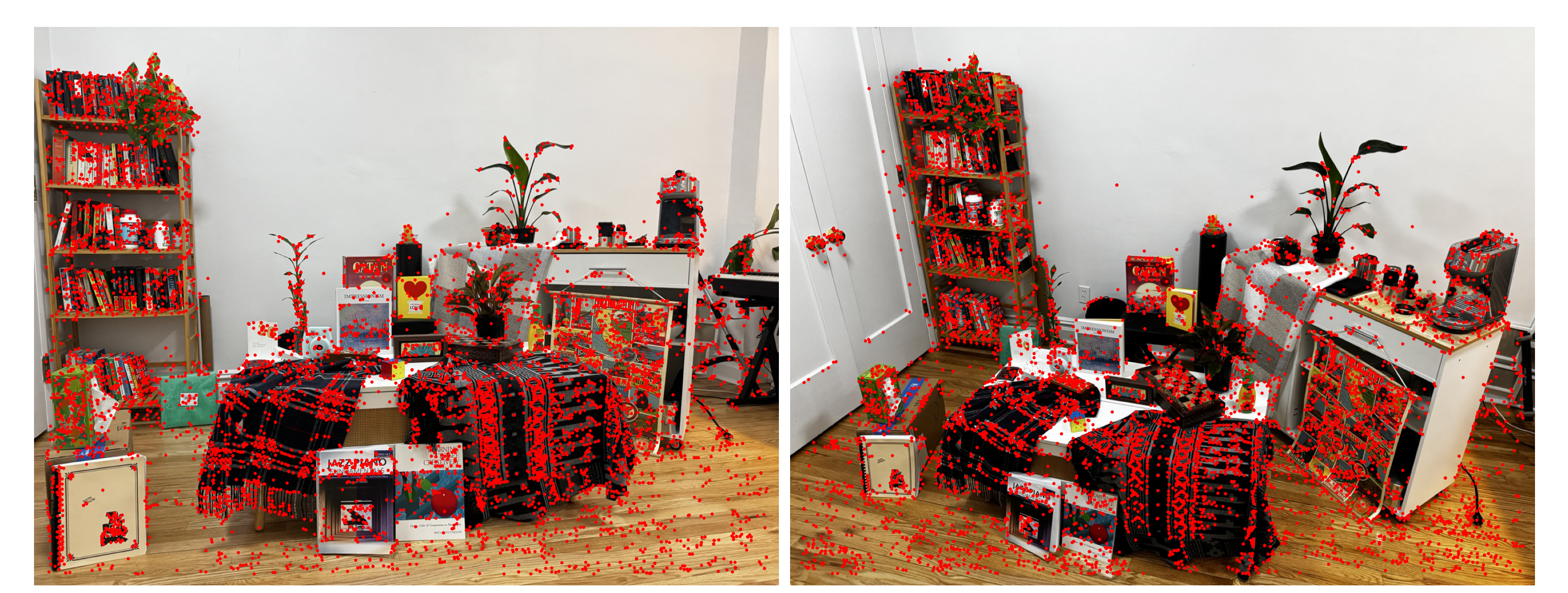
SIFT features detected in both images, side-by-side

Step 3: Feature Matching (15 points)

In HW2, we created feature descriptors then subsequently did an $n^2$ search between the features in image 1 and image 2, using a metric like SSD or NCC to compare the features. We also applied the ratio test between the 1NN and 2NN features in image 2 for a feature in image 1. This is the nearest neighbor distance ratio (NNDR).

In this HW, the OpenCV SIFT API cv2.SIFT_create directly returns keypoints and feature descriptors––all that’s left is to match the features between these images. We use an L2 loss to compare these features, as is typically done with SIFT. Since you’ve already implemented this in HW2, we provide code that uses a C++-optimized feature matching algorithm: cv2.BFMatcher. You still need to provide an NNDR threshold, like we did in HW2.

[Deliverables]

• Show the histogram of NNDR’s for the scene. Indicate what threshold you used.
• Show the top 5 feature descriptors according to NNDR.
• Visualize side-by-side the correspondences. It’s okay if it’s slightly unclear what corresponds to what.

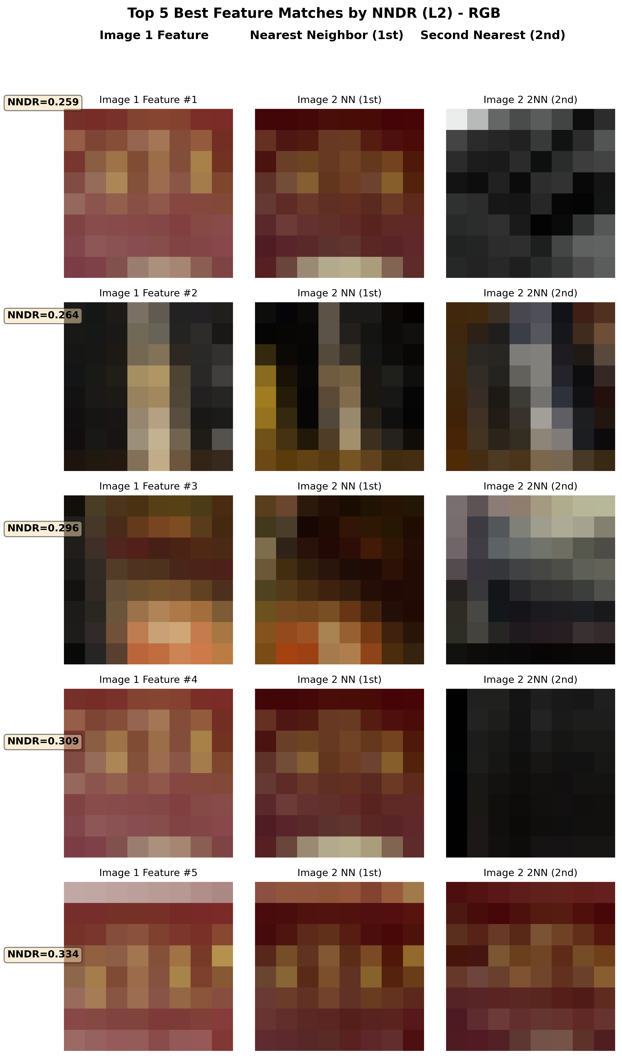
Top 5 feature matches by NNDR

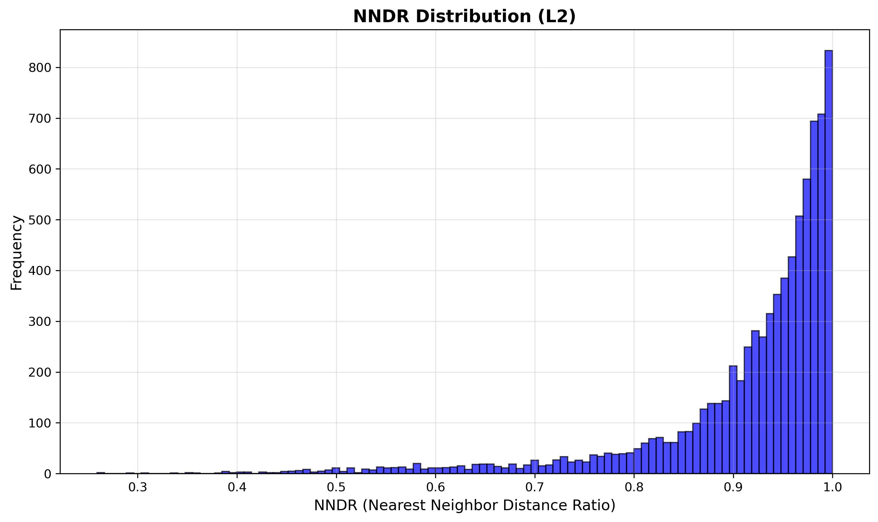
NNDR histogram

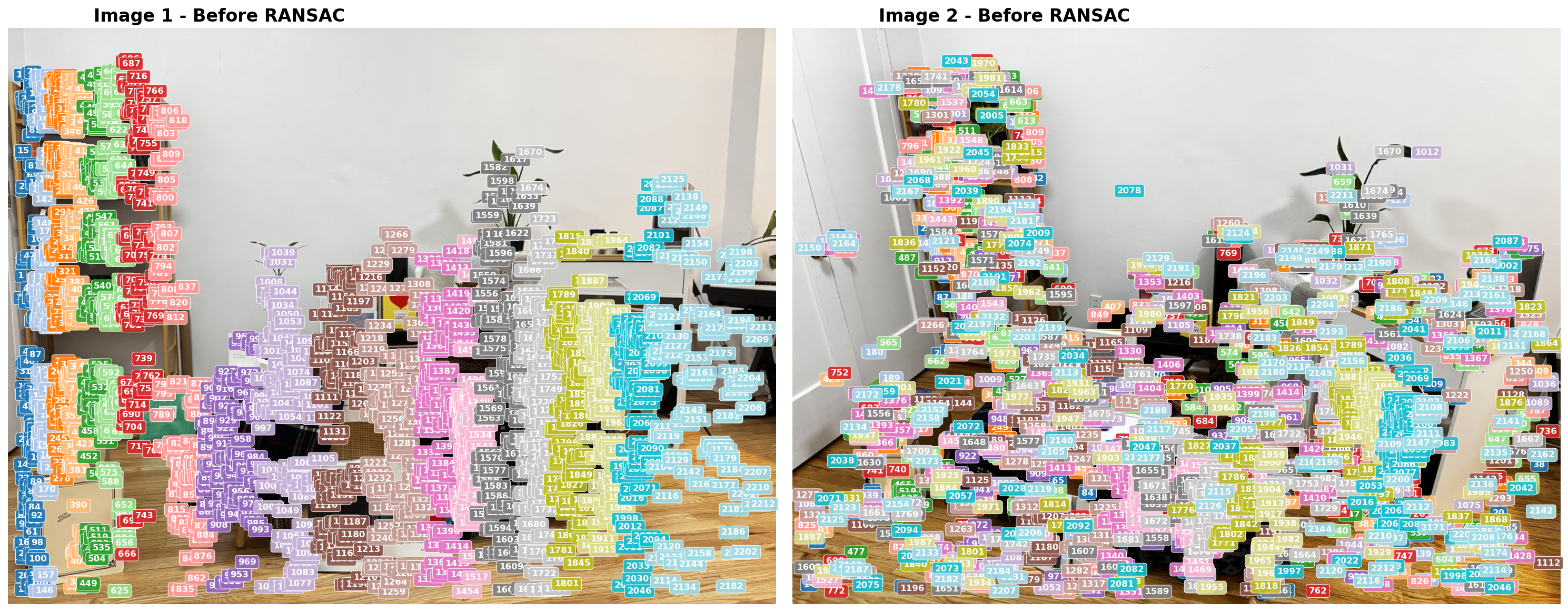
Matched correspondences

Step 4: RANSAC to estimate R and t (45 points)

Now we must estimate the rotation matrix $R$ and translation vector $t$ that relate camera 2 (from image 2) to camera 1 (from image 1). We treat camera 1’s center as the origin. We do this via RANSAC and epipolar geometry. You are not expected to understand the epipolar geometry well, but you are expected to understand how RANSAC can be used as a general method to estimate the parameters of some mathematical model for which we have data that contains inliers and outliers. As such, you will be implementing parts of RANSAC in this HW.

The mathematical model we hope to estimate is the rotation and translation that relates these two images. Using epipolar geometry, there is an essential matrix $E$ that relates the features between the images. We can use RANSAC to estimate $E$ and decompose it into $R$ and $t$ that relate the cameras.

Note: you’ll notice in our algorithm that we sample eight points, not five. Even though there are only 5 unknown variables (and therefore only 5 correspondences are needed to learn $E$), the five-point algorithm requires solving a tenth-degree polynomial and the solution’s implementation can be tricky to follow. Instead, we provide an implementation for the eight-point algorithm which fits $E$ on eight points with a linear system of equations. This is all abstracted away from you but you’re welcome to dig into the implementation if curious.

Algorithm 1: RANSAC for Essential Matrix Estimation

Input: correspondence pairs $\{(p_1^i, p_2^i)\}_{i=1}^{N}$ from Step 3, camera intrinsics $K$, number of iterations $T$, Sampson distance threshold $\epsilon$

Output: rotation $R$, translation $t$, inlier mask

1:   best_inliers ← 0;   $E^*$ ← None

2:   for iter = 1 to $T$ do

3:   Randomly sample 8 correspondences

4:   Estimate essential matrix $E$ from the 8 samples

5:   Decompose $E$ into 4 candidate $(R, t)$ pairs and run cheirality check on the sample

6:   if no valid $(R, t)$ found, continue to next iteration

7:   Compute inliers over all correspondences: $\;\mathcal{I} \leftarrow \{i : d_{\text{Sampson}}^2(E,\, p_1^i,\, p_2^i) < \epsilon \}$

8:   if $|\mathcal{I}|$ > best_inliers then

9:   best_inliers ← $|\mathcal{I}|$;   save $E^*$

10:   end if

11:   end for

12:   if best_inliers > 8 then

13:   Recompute inliers $\mathcal{I}^*$ from $E^*$ over all correspondences

14:   Re-estimate $E$ from $\mathcal{I}^*$

15:   Recover $R, t$ from refined $E$ via decomposition + cheirality

16:   end if

17:   return $R, t$, inlier mask

[Hints]

• There is a chance that post-loop refinement may not improve your RANSAC outputs. It is okay to decide not to do post-loop refinement, just make sure to mention whether or not you did.
• Your epipolar lines in the outputted step4_epipolar_lines.png visualization should look something like the image below: each feature should lie on or close to the epipolar line of the same color. You can also visualize these lines in step5_pipeline_grid.png.

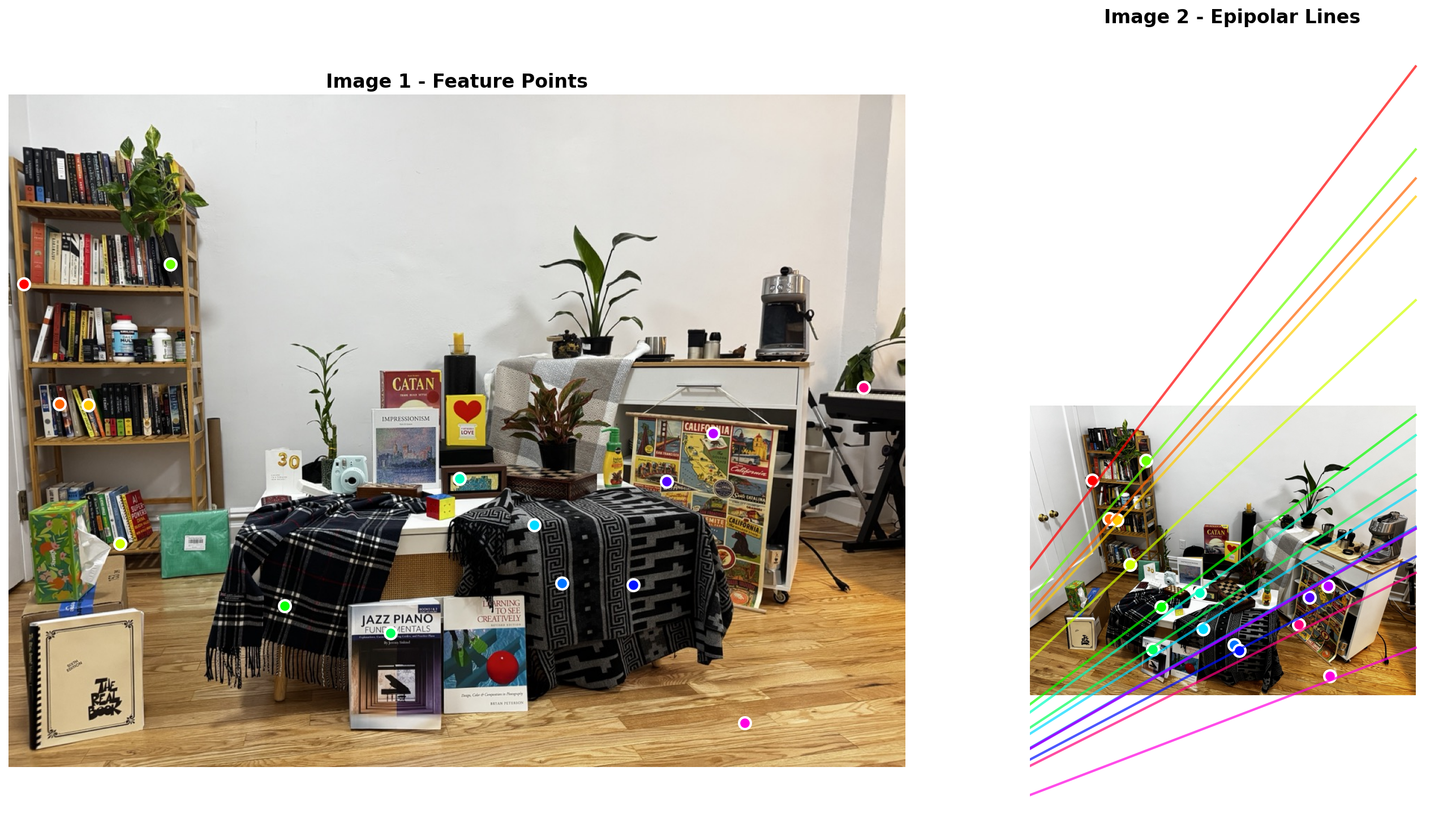
Epipolar lines: each feature should lie on or near the epipolar line of the same color

[Deliverables]

• Complete the ransac.py implementation.
• Report RANSAC parameters used: number of iterations $T$, Sampson distance threshold $\epsilon$, and the final number of inliers found.
• Visualize the RANSAC convergence (best inlier count over iterations).
• Visualize the matched correspondences after RANSAC (inliers only).

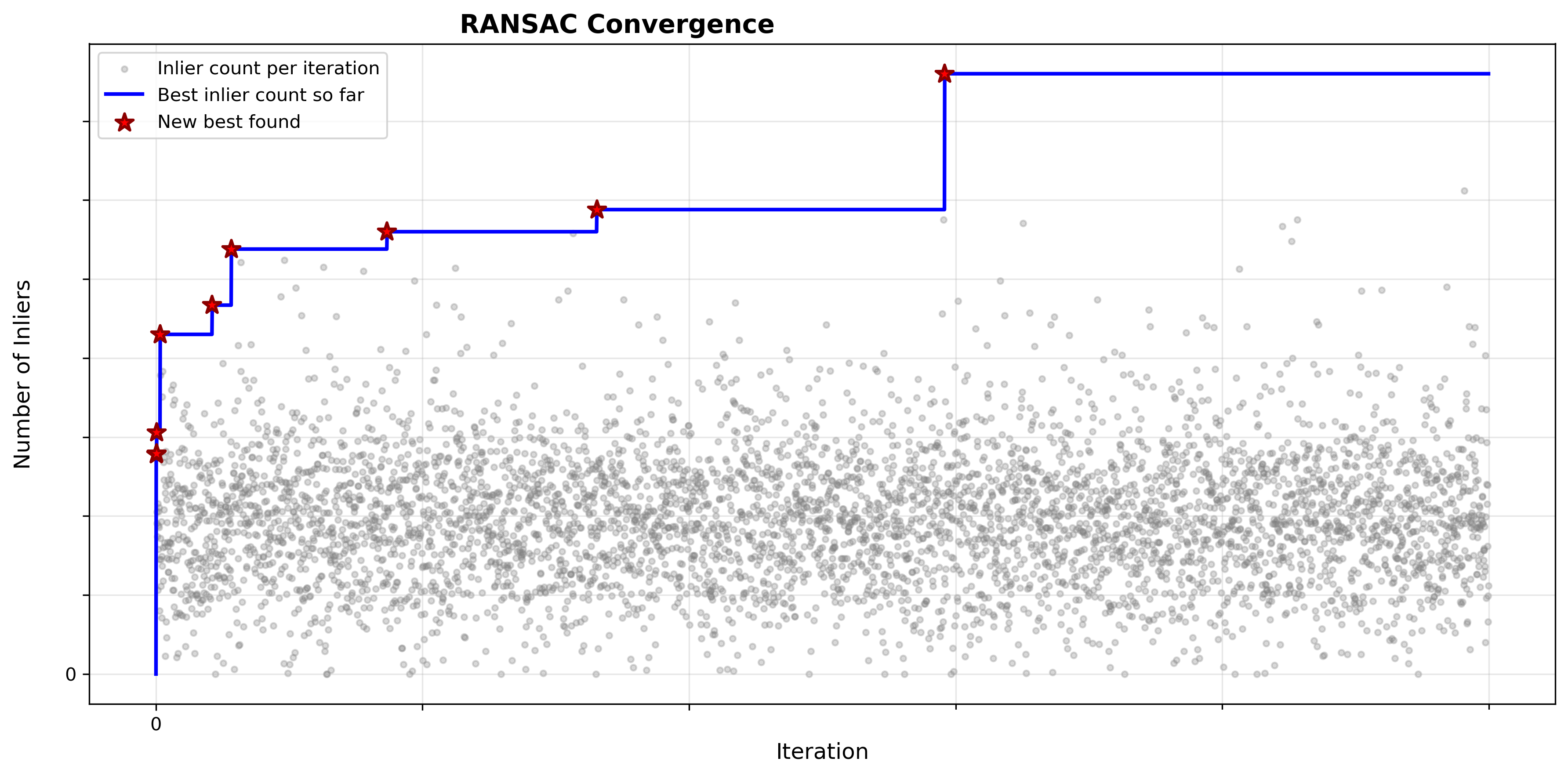
RANSAC convergence: best inlier count over iterations

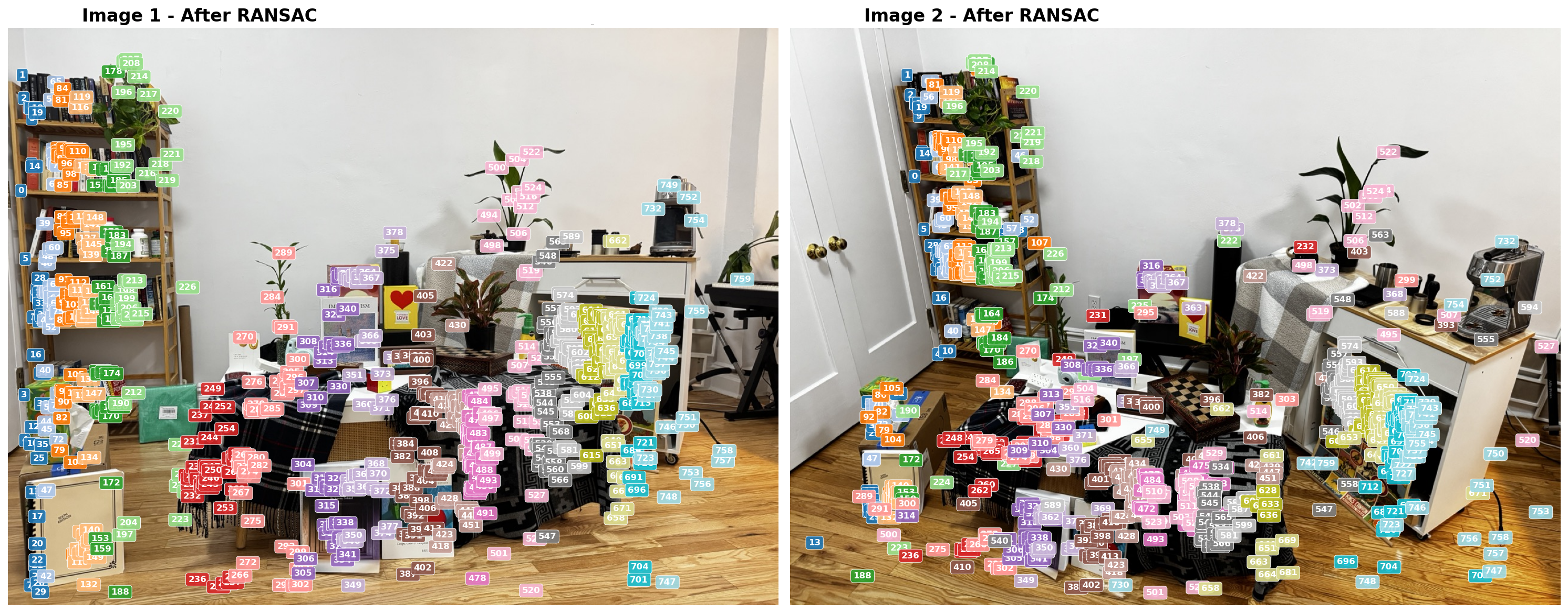
Feature correspondences after RANSAC (inliers only)

Step 5: Triangulating Inliers to generate Point Cloud (10 points, done for you)

Now that we have the camera poses ($R$ and $t$ from Step 4) and the inlier correspondences, we can recover the 3D positions of the matched points via triangulation. This part is already done for you, but you will need to load the outputs into Viser and show screenshots of the sparse point cloud. If the previous steps are implemented properly and main.py executes, a viser command will be outputted at the very end of the script.

[Hints]

When debugging, compare your point cloud with the input images and ask yourself:

• Are your inliers after RANSAC good enough? Do they actually correspond to the same feature across the images?
• Do the different surfaces at different depths seem right?
• Do planar surfaces in the image look planar in the point cloud?
• Do the cameras look right? Is camera 2 rotated and translated in a way consistent with the real scene?

Additionally:

• You probably don’t want a super strict NNDR threshold: we’re using RANSAC as a geometry-grounded outlier rejection method, and therefore don’t need the NNDR filtering to remove too many points. In fact: we want to strike a balance of having enough points passed into step 4 so that, after RANSAC, enough points survive to have a decent point cloud.
• Do your epipolar lines look correct?
• You shouldn’t need to touch the triangulation-related parameters in the config, but they are accessible in case you’d like to adjust them
• Triangulation will cause you to lose some points from your initial set of RANSAC inliers. This is expected. For reference: staff solution lost ~10 points after performing triangulation.

[Deliverables]

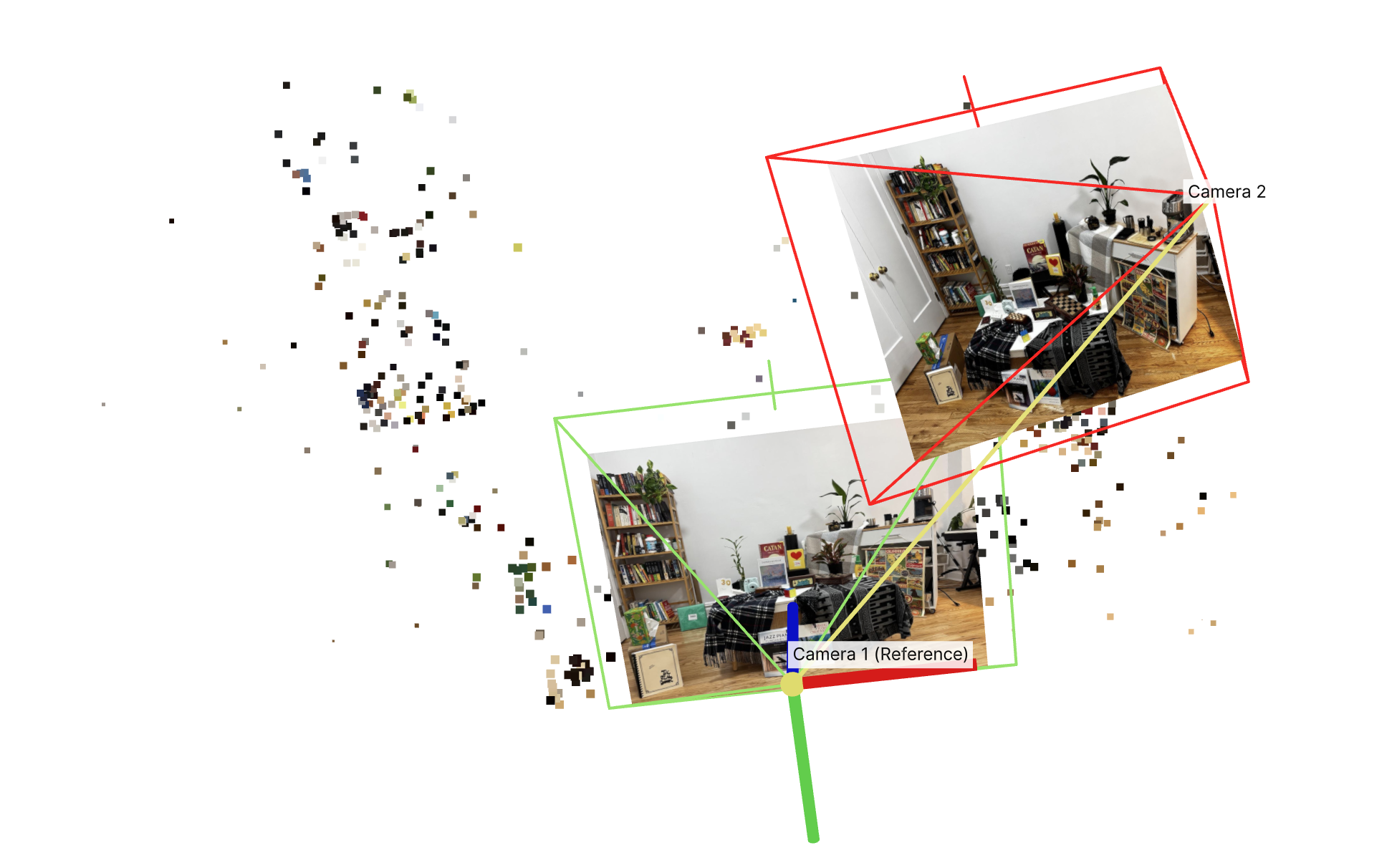
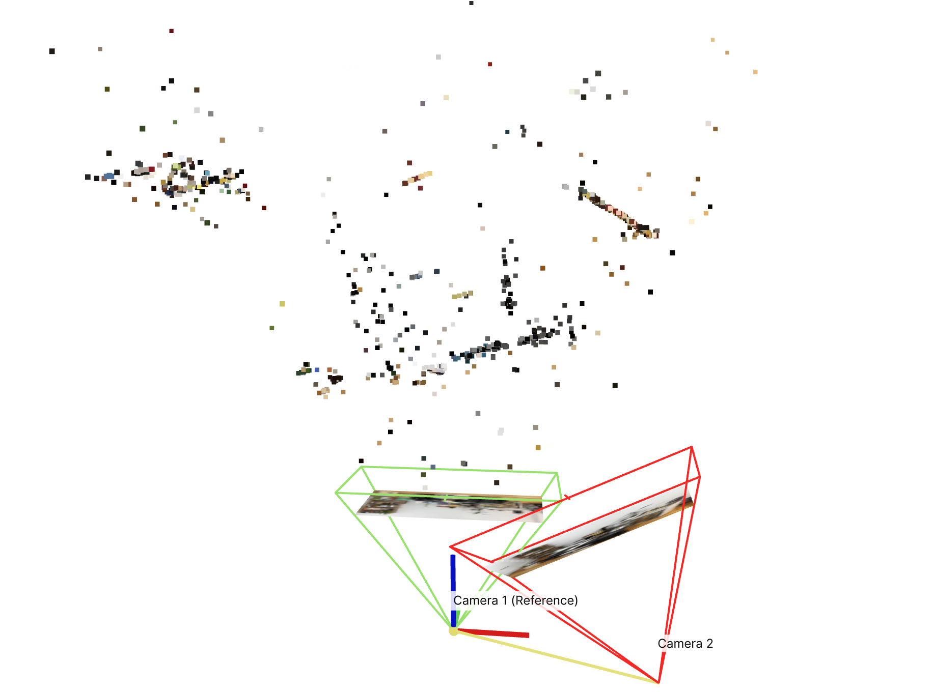
3 screenshots of the Viser server showing the point cloud from different angles:

• All 3 of them should show the cameras so we can observe the rotation + translation that relates them and have a reference across the 3 images.
• All 3 of them should have a caption/description of what the identifiable ‘landmarks’ from the original images are visible, since your point cloud will likely be sparse and hard to understand at first glance.
  • You may have more or less points than the staff’s point cloud shown. As long as you can justify that your estimated geometry is correct, you’ll receive points.

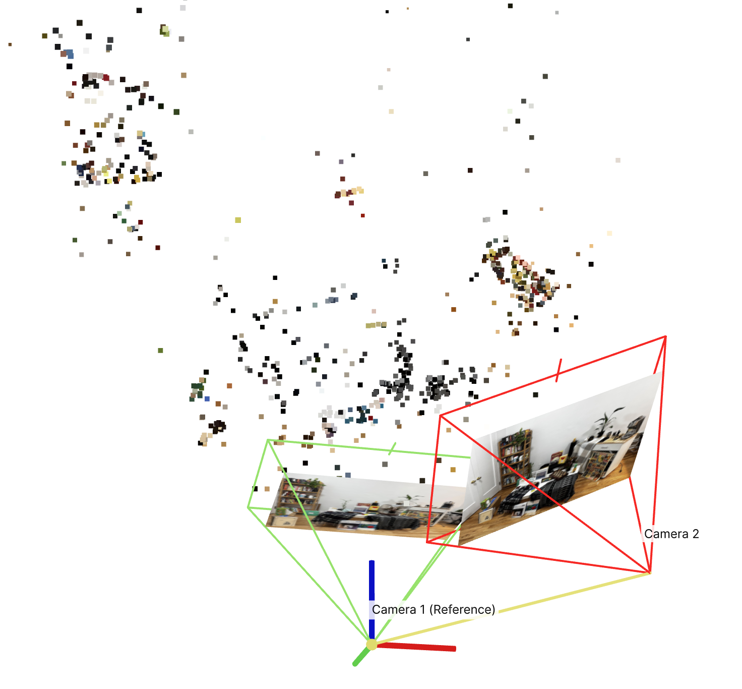
... I see bookshelf, poster, coffee table ...

... the right camera looks correctly positioned to the top right of camera 1, with correct rotation applied ...

... the poster looks planar from this angle, as expected ...

Assignment Deliverables

As with HW1 and HW2, you must submit both your code and a webpage written as an index.html with pointers to images/assets. You must also submit a README.md file that outlines how to run your code. Lastly, submit a PDF version of your webpage. Failure to submit any of these will result in lost points.

For the staff-provided images, report the following:

• Your random seed chosen
• Camera intrinsics matrix $K$ used in the pipeline
• SIFT number of points detected
• Feature matching nearest neighbor distance ratio (NNDR) threshold used
• RANSAC parameters:
  • number of RANSAC iterations
  • $\epsilon$ parameter used
• Any other staff-provided parameters that you modified.
• Visualizations of:
  • SIFT features
  • NNDR histogram, with threshold overlaid
  • Top 5 features matched, ranked by NNDR
  • Correspondences between image 1 and 2 before RANSAC
  • Correspondences between image 1 and 2 after RANSAC
  • RANSAC convergence.
  • At least 3 screenshots of sparse point cloud with ‘landmarks’ described.

Extra Credit

Capture your own scene (10 points, competition)

You are required to use the staff-provided images (provided in the overview) for full credit on this assignment.

For extra credit, reconstruct your own scene with our simple SfM pipeline on 2 images of your own. You get 10 points if you can get a decent reconstruction, and we will also be voting on the best custom scenes! For this section, stick to the current pipeline. You are allowed to modify: scene contents (via the photos you take), image resolution, and config hyperparameters.

You’ll need to provide the parameters for your own camera used. If this is difficult to access online, you can try accessing the image metadata and recover the parameters.

Advice:

• Lock the exposure and focus of your camera before taking photos. This will make it easier to find common features across the scene images.
• Choose a scene with multiple levels of depth (2+). Failing to do so will cause the model to only pick planar correspondences, which don’t exhibit much disparity/parallax across camera angles. This makes it significantly harder to determine the geometry that relates these two photos (since we don’t exhibit much change between them). Thus, we want a scene with varying levels of depth so that we see parallax at varying distances.
  • this also means that we don’t only want to rotate our camera but translate as well. You will need to find a sweet spot between how much or how little translation to use. In a realistic pipeline you’d have ≫ 2 images taken and wouldn’t have to worry about this as much.
• Choose a scene with lots of textured objects. The SIFT feature descriptor used is targeting textures and your pipeline’s performance will markedly increase with the number of textured objects (ideally with textures at different distances in the scene).

More details on competition to come.

Improve the staff solution (class competition)

Improve on the staff-provided scene! You are allowed to make changes as long as they maintain our 6-step pipeline. This includes but isn’t strictly limited to adjusting the hyperparameters. Since it’s not super well-defined what’s a “better” point cloud, we’ll do a user-study: we’ll do a class vote and vote for the best results!

More details on competition to come.

---

Appendix with math explanations will be released soon.

Acknowledgements

This assignment was created by Ryan Tabrizi with helpful feedback from Jordan Lin and Aleksander Holynski.